Cleaning and wrangling data
Contents
Cleaning and wrangling data
Overview
This chapter is centered around defining tidy data—a data format that is suitable for analysis—and the tools needed to transform raw data into this format. This will be presented in the context of a real-world data science application, providing more practice working through a whole case study.
Chapter learning objectives
By the end of the chapter, readers will be able to do the following:
Define the term “tidy data”.
Discuss the advantages of storing data in a tidy data format.
Define what lists, series and data frames are in Python, and describe how they relate to each other.
Describe the common types of data in Python and their uses.
Recall and use the following functions for their intended data wrangling tasks:
.agg.apply.assign.groupby.melt.pivot.str.split
Recall and use the following operators for their intended data wrangling tasks:
==inandordf[].iloc[].loc[]
Data frames, series, and lists
In Chapters intro and reading, data frames were the focus:
we learned how to import data into Python as a data frame, and perform basic operations on data frames in Python.
In the remainder of this book, this pattern continues. The vast majority of tools we use will require
that data are represented as a pandas data frame in Python. Therefore, in this section,
we will dig more deeply into what data frames are and how they are represented in Python.
This knowledge will be helpful in effectively utilizing these objects in our data analyses.
What is a data frame?
A data frame \index{data frame!definition} is a table-like structure for storing data in Python. Data frames are important to learn about because most data that you will encounter in practice can be naturally stored as a table. In order to define data frames precisely, we need to introduce a few technical terms:
variable: a \index{variable} characteristic, number, or quantity that can be measured.
observation: all \index{observation} of the measurements for a given entity.
value: a \index{value} single measurement of a single variable for a given entity.
Given these definitions, a data frame is a tabular data structure in Python that is designed to store observations, variables, and their values. Most commonly, each column in a data frame corresponds to a variable, and each row corresponds to an observation. For example, Fig. 12 displays a data set of city populations. Here, the variables are “region, year, population”; each of these are properties that can be collected or measured. The first observation is “Toronto, 2016, 2235145”; these are the values that the three variables take for the first entity in the data set. There are 13 entities in the data set in total, corresponding to the 13 rows in Fig. 12.
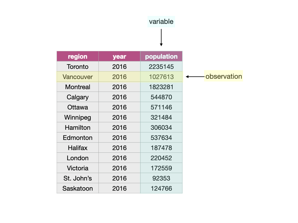
Fig. 12 A data frame storing data regarding the population of various regions in Canada. In this example data frame, the row that corresponds to the observation for the city of Vancouver is colored yellow, and the column that corresponds to the population variable is colored blue.
What is a series?
In Python, pandas series are arrays with labels. They are strictly 1-dimensional and can contain any data type (integers, strings, floats, etc), including a mix of them (objects);
Python has several different basic data types, as shown in Table 3.
You can create a pandas series using the pd.Series() function. For
example, to create the vector region as shown in
Fig. 13, you can write:
import pandas as pd
region = pd.Series(["Toronto", "Montreal", "Vancouver", "Calgary", "Ottawa"])
region
0      Toronto
1     Montreal
2    Vancouver
3      Calgary
4       Ottawa
dtype: object
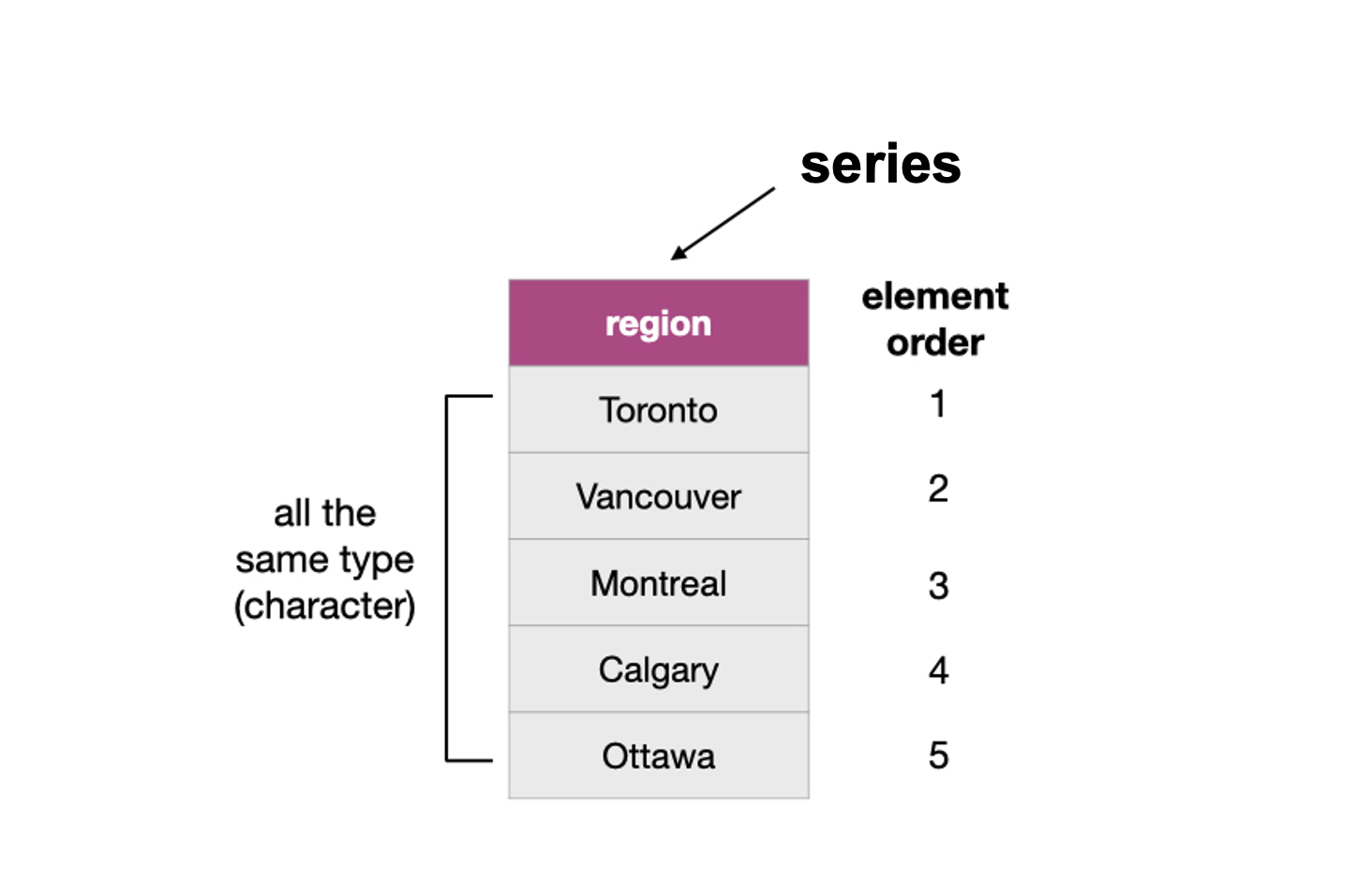
Fig. 13 Example of a pandas series whose type is string.
\newpage
English name |
Type name |
Type Category |
Description |
Example |
|---|---|---|---|---|
integer |
|
Numeric Type |
positive/negative whole numbers |
|
floating point number |
|
Numeric Type |
real number in decimal form |
|
boolean |
|
Boolean Values |
true or false |
|
string |
|
Sequence Type |
text |
|
list |
|
Sequence Type |
a collection of objects - mutable & ordered |
|
tuple |
|
Sequence Type |
a collection of objects - immutable & ordered |
|
dictionary |
|
Mapping Type |
mapping of key-value pairs |
|
none |
|
Null Object |
represents no value |
|
\index{data types}
\index{character}\index{chr|see{character}}
\index{integer}\index{int|see{integer}}
\index{double}\index{dbl|see{double}}
\index{logical}\index{lgl|see{logical}}
\index{factor}\index{fct|see{factor}}
It is important in Python to make sure you represent your data with the correct type.
Many of the pandas functions we use in this book treat
the various data types differently. You should use integers and float types
(which both fall under the “numeric” umbrella type) to represent numbers and perform
arithmetic. Strings are used to represent data that should
be thought of as “text”, such as words, names, paths, URLs, and more.
There are other basic data types in Python, such as set
and complex, but we do not use these in this textbook.
What is a list?
Lists \index{list} are built-in objects in Python that have multiple, ordered elements.
pandas series can be treated as lists with labels (indices).
What does this have to do with data frames?
A data frame \index{data frame!definition} is really just series stuck together that follows two rules:
Each element itself is a series.
Each element (series) must have the same length.
Not all columns in a data frame need to be of the same type. Fig. 14 shows a data frame where the columns are series of different types.
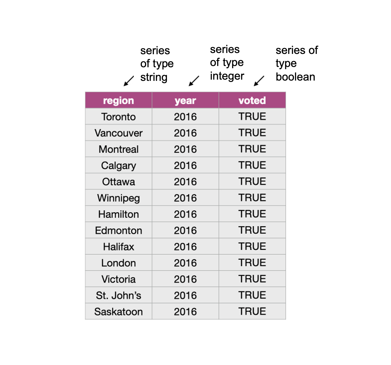
Fig. 14 Data frame and vector types.
Note: You can use the function
type\index{class} on a data object. For example we can check the class of the Canadian languages data set,can_lang, we worked with in the previous chapters and we see it is apandas.core.frame.DataFrame.
can_lang = pd.read_csv("data/can_lang.csv")
type(can_lang)
---------------------------------------------------------------------------
FileNotFoundError                         Traceback (most recent call last)
Input In [10], in <cell line: 1>()
----> 1 can_lang = pd.read_csv("data/can_lang.csv")
      2 type(can_lang)

File ~/opt/miniconda3/envs/dsci/lib/python3.9/site-packages/pandas/util/_decorators.py:311, in deprecate_nonkeyword_arguments.<locals>.decorate.<locals>.wrapper(*args, **kwargs)
    305 if len(args) > num_allow_args:
    306     warnings.warn(
    307         msg.format(arguments=arguments),
    308         FutureWarning,
    309         stacklevel=stacklevel,
    310     )
--> 311 return func(*args, **kwargs)

File ~/opt/miniconda3/envs/dsci/lib/python3.9/site-packages/pandas/io/parsers/readers.py:680, in read_csv(filepath_or_buffer, sep, delimiter, header, names, index_col, usecols, squeeze, prefix, mangle_dupe_cols, dtype, engine, converters, true_values, false_values, skipinitialspace, skiprows, skipfooter, nrows, na_values, keep_default_na, na_filter, verbose, skip_blank_lines, parse_dates, infer_datetime_format, keep_date_col, date_parser, dayfirst, cache_dates, iterator, chunksize, compression, thousands, decimal, lineterminator, quotechar, quoting, doublequote, escapechar, comment, encoding, encoding_errors, dialect, error_bad_lines, warn_bad_lines, on_bad_lines, delim_whitespace, low_memory, memory_map, float_precision, storage_options)
    665 kwds_defaults = _refine_defaults_read(
    666     dialect,
    667     delimiter,
   (...)
    676     defaults={"delimiter": ","},
    677 )
    678 kwds.update(kwds_defaults)
--> 680 return _read(filepath_or_buffer, kwds)

File ~/opt/miniconda3/envs/dsci/lib/python3.9/site-packages/pandas/io/parsers/readers.py:575, in _read(filepath_or_buffer, kwds)
    572 _validate_names(kwds.get("names", None))
    574 # Create the parser.
--> 575 parser = TextFileReader(filepath_or_buffer, **kwds)
    577 if chunksize or iterator:
    578     return parser

File ~/opt/miniconda3/envs/dsci/lib/python3.9/site-packages/pandas/io/parsers/readers.py:933, in TextFileReader.__init__(self, f, engine, **kwds)
    930     self.options["has_index_names"] = kwds["has_index_names"]
    932 self.handles: IOHandles | None = None
--> 933 self._engine = self._make_engine(f, self.engine)

File ~/opt/miniconda3/envs/dsci/lib/python3.9/site-packages/pandas/io/parsers/readers.py:1217, in TextFileReader._make_engine(self, f, engine)
   1213     mode = "rb"
   1214 # error: No overload variant of "get_handle" matches argument types
   1215 # "Union[str, PathLike[str], ReadCsvBuffer[bytes], ReadCsvBuffer[str]]"
   1216 # , "str", "bool", "Any", "Any", "Any", "Any", "Any"
-> 1217 self.handles = get_handle(  # type: ignore[call-overload]
   1218     f,
   1219     mode,
   1220     encoding=self.options.get("encoding", None),
   1221     compression=self.options.get("compression", None),
   1222     memory_map=self.options.get("memory_map", False),
   1223     is_text=is_text,
   1224     errors=self.options.get("encoding_errors", "strict"),
   1225     storage_options=self.options.get("storage_options", None),
   1226 )
   1227 assert self.handles is not None
   1228 f = self.handles.handle

File ~/opt/miniconda3/envs/dsci/lib/python3.9/site-packages/pandas/io/common.py:789, in get_handle(path_or_buf, mode, encoding, compression, memory_map, is_text, errors, storage_options)
    784 elif isinstance(handle, str):
    785     # Check whether the filename is to be opened in binary mode.
    786     # Binary mode does not support 'encoding' and 'newline'.
    787     if ioargs.encoding and "b" not in ioargs.mode:
    788         # Encoding
--> 789         handle = open(
    790             handle,
    791             ioargs.mode,
    792             encoding=ioargs.encoding,
    793             errors=errors,
    794             newline="",
    795         )
    796     else:
    797         # Binary mode
    798         handle = open(handle, ioargs.mode)

FileNotFoundError: [Errno 2] No such file or directory: 'data/can_lang.csv'
Lists, Series and DataFrames are basic types of data structure in Python, which are core to most data analyses. We summarize them in Table 4. There are several other data structures in the Python programming language (e.g., matrices), but these are beyond the scope of this book.
Data Structure |
Description |
|---|---|
list |
An 1D ordered collection of values that can store multiple data types at once. |
Series |
An 1D ordered collection of values with labels that can store multiple data types at once. |
DataFrame |
A 2D labeled data structure with columns of potentially different types. |
Tidy data
There are many ways a tabular data set can be organized. This chapter will focus on introducing the tidy data \index{tidy data!definition} format of organization and how to make your raw (and likely messy) data tidy. A tidy data frame satisfies the following three criteria [Wickham, 2014]:
each row is a single observation,
each column is a single variable, and
each value is a single cell (i.e., its entry in the data frame is not shared with another value).
Fig. 15 demonstrates a tidy data set that satisfies these three criteria.
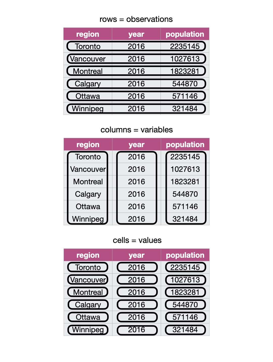
Fig. 15 Tidy data satisfies three criteria.
There are many good reasons for making sure your data are tidy as a first step in your analysis.
The most important is that it is a single, consistent format that nearly every function
in the pandas recognizes. No matter what the variables and observations
in your data represent, as long as the data frame \index{tidy data!arguments for}
is tidy, you can manipulate it, plot it, and analyze it using the same tools.
If your data is not tidy, you will have to write special bespoke code
in your analysis that will not only be error-prone, but hard for others to understand.
Beyond making your analysis more accessible to others and less error-prone, tidy data
is also typically easy for humans to interpret. Given these benefits,
it is well worth spending the time to get your data into a tidy format
upfront. Fortunately, there are many well-designed pandas data
cleaning/wrangling tools to help you easily tidy your data. Let’s explore them
below!
Note: Is there only one shape for tidy data for a given data set? Not necessarily! It depends on the statistical question you are asking and what the variables are for that question. For tidy data, each variable should be its own column. So, just as it’s essential to match your statistical question with the appropriate data analysis tool, it’s important to match your statistical question with the appropriate variables and ensure they are represented as individual columns to make the data tidy.
Tidying up: going from wide to long using .melt
One task that is commonly performed to get data into a tidy format \index{pivot_longer} is to combine values that are stored in separate columns, but are really part of the same variable, into one. Data is often stored this way because this format is sometimes more intuitive for human readability and understanding, and humans create data sets. In Fig. 16, the table on the left is in an untidy, “wide” format because the year values (2006, 2011, 2016) are stored as column names. And as a consequence, the values for population for the various cities over these years are also split across several columns.
For humans, this table is easy to read, which is why you will often find data
stored in this wide format. However, this format is difficult to work with
when performing data visualization or statistical analysis using Python. For
example, if we wanted to find the latest year it would be challenging because
the year values are stored as column names instead of as values in a single
column. So before we could apply a function to find the latest year (for
example, by using max), we would have to first extract the column names
to get them as a list and then apply a function to extract the latest year.
The problem only gets worse if you would like to find the value for the
population for a given region for the latest year. Both of these tasks are
greatly simplified once the data is tidied.
Another problem with data in this format is that we don’t know what the numbers under each year actually represent. Do those numbers represent population size? Land area? It’s not clear. To solve both of these problems, we can reshape this data set to a tidy data format by creating a column called “year” and a column called “population.” This transformation—which makes the data “longer”—is shown as the right table in Fig. 16.
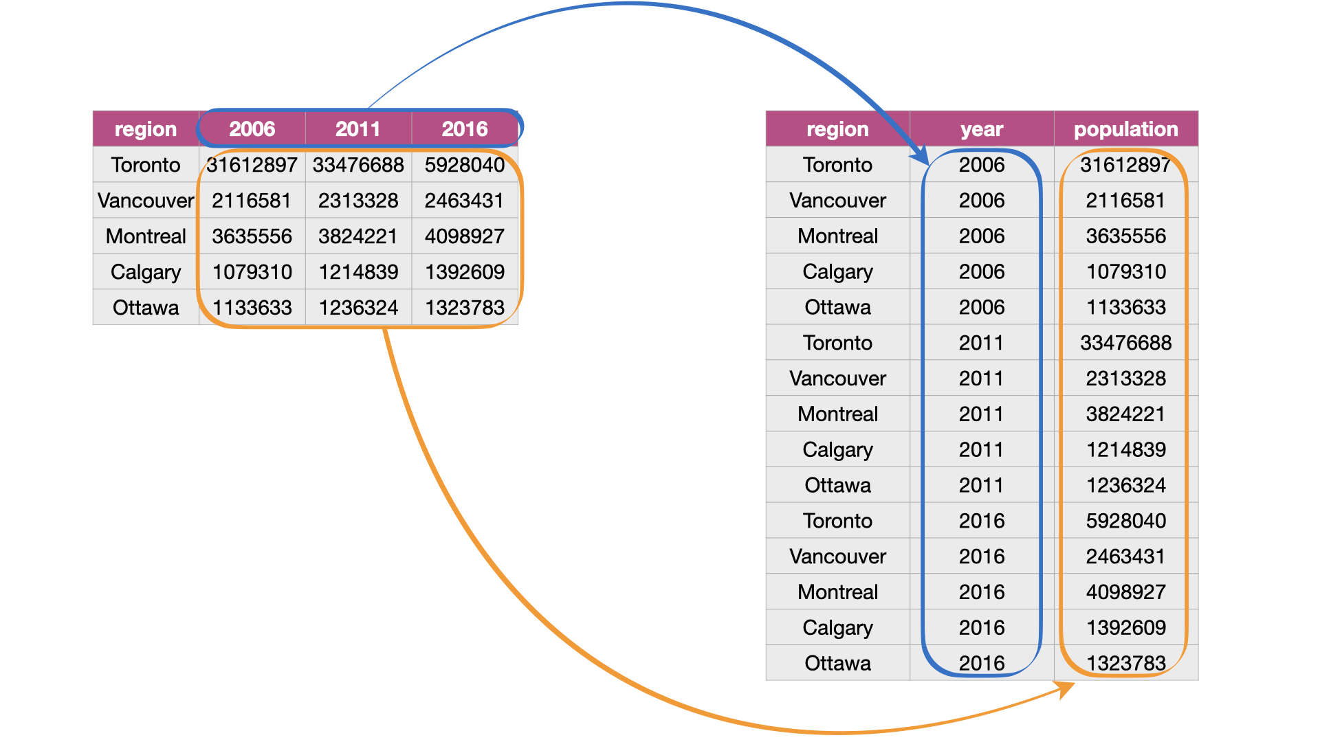
Fig. 16 Melting data from a wide to long data format.
We can achieve this effect in Python using the .melt function from the pandas package.
The .melt function combines columns,
and is usually used during tidying data
when we need to make the data frame longer and narrower.
To learn how to use .melt, we will work through an example with the
region_lang_top5_cities_wide.csv data set. This data set contains the
counts of how many Canadians cited each language as their mother tongue for five
major Canadian cities (Toronto, Montréal, Vancouver, Calgary and Edmonton) from
the 2016 Canadian census. \index{Canadian languages}
To get started,
we will use pd.read_csv to load the (untidy) data.
lang_wide = pd.read_csv("data/region_lang_top5_cities_wide.csv")
lang_wide
| category | language | Toronto | Montréal | Vancouver | Calgary | Edmonton | |
|---|---|---|---|---|---|---|---|
| 0 | Aboriginal languages | Aboriginal languages, n.o.s. | 80 | 30 | 70 | 20 | 25 |
| 1 | Non-Official & Non-Aboriginal languages | Afrikaans | 985 | 90 | 1435 | 960 | 575 |
| 2 | Non-Official & Non-Aboriginal languages | Afro-Asiatic languages, n.i.e. | 360 | 240 | 45 | 45 | 65 |
| 3 | Non-Official & Non-Aboriginal languages | Akan (Twi) | 8485 | 1015 | 400 | 705 | 885 |
| 4 | Non-Official & Non-Aboriginal languages | Albanian | 13260 | 2450 | 1090 | 1365 | 770 |
| ... | ... | ... | ... | ... | ... | ... | ... |
| 209 | Non-Official & Non-Aboriginal languages | Wolof | 165 | 2440 | 30 | 120 | 130 |
| 210 | Aboriginal languages | Woods Cree | 5 | 0 | 20 | 10 | 155 |
| 211 | Non-Official & Non-Aboriginal languages | Wu (Shanghainese) | 5290 | 1025 | 4330 | 380 | 235 |
| 212 | Non-Official & Non-Aboriginal languages | Yiddish | 3355 | 8960 | 220 | 80 | 55 |
| 213 | Non-Official & Non-Aboriginal languages | Yoruba | 3380 | 210 | 190 | 1430 | 700 |
214 rows × 7 columns
What is wrong with the untidy format above?
The table on the left in Fig. 17
represents the data in the “wide” (messy) format.
From a data analysis perspective, this format is not ideal because the values of
the variable region (Toronto, Montréal, Vancouver, Calgary and Edmonton)
are stored as column names. Thus they
are not easily accessible to the data analysis functions we will apply
to our data set. Additionally, the mother tongue variable values are
spread across multiple columns, which will prevent us from doing any desired
visualization or statistical tasks until we combine them into one column. For
instance, suppose we want to know the languages with the highest number of
Canadians reporting it as their mother tongue among all five regions. This
question would be tough to answer with the data in its current format.
We could find the answer with the data in this format,
though it would be much easier to answer if we tidy our
data first. If mother tongue were instead stored as one column,
as shown in the tidy data on the right in
Fig. 17,
we could simply use one line of code (df["mother_tongue"].max())
to get the maximum value.
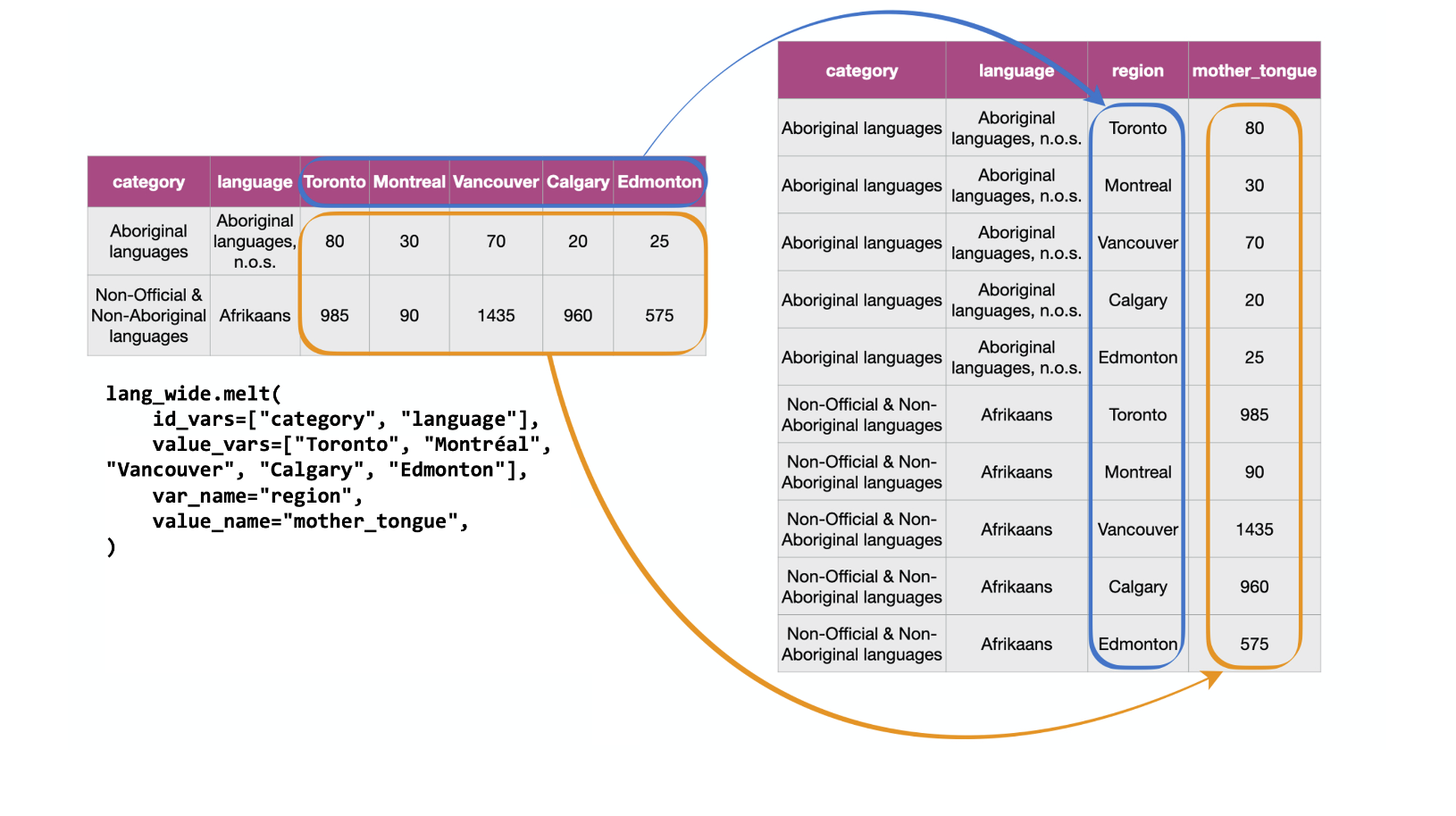
Fig. 17 Going from wide to long with the .melt function.
Fig. 18 details the arguments that we need to specify
in the .melt function to accomplish this data transformation.
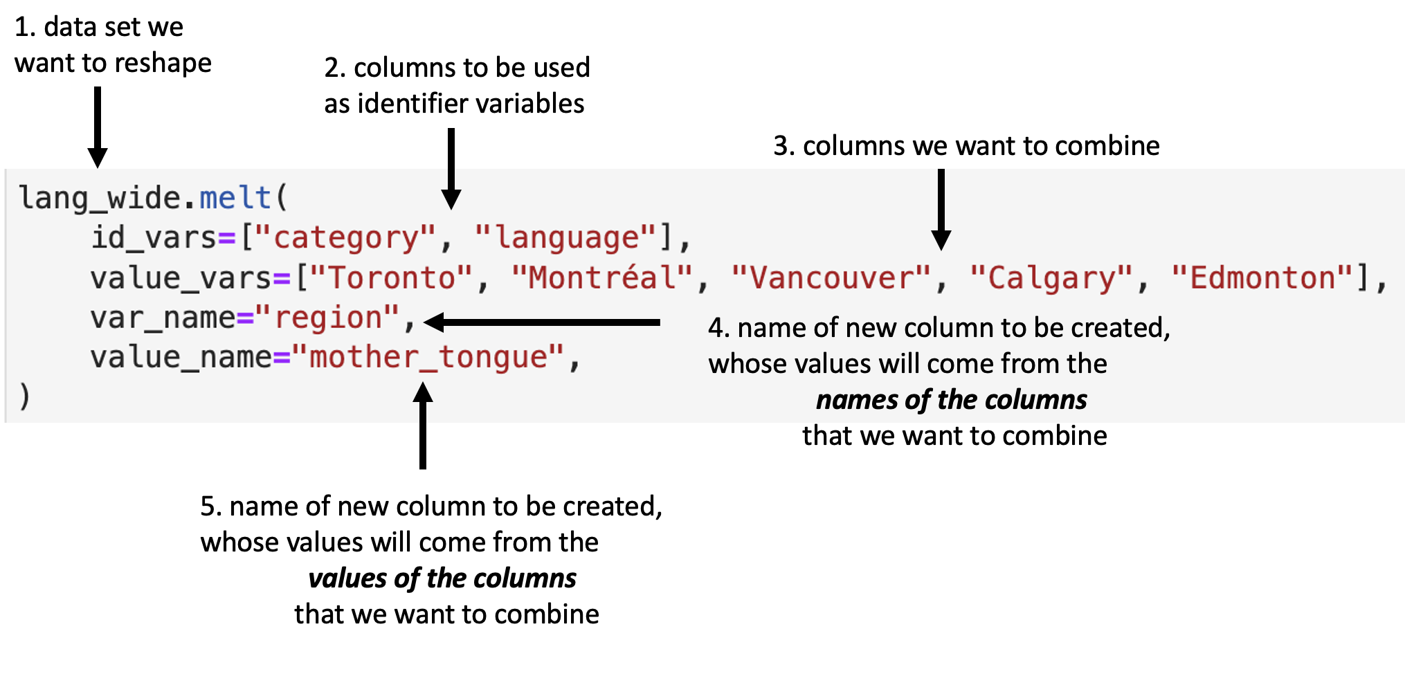
Fig. 18 Syntax for the melt function.
We use .melt to combine the Toronto, Montréal,
Vancouver, Calgary, and Edmonton columns into a single column called region,
and create a column called mother_tongue that contains the count of how many
Canadians report each language as their mother tongue for each metropolitan
area. We specify value_vars to be all
the columns between Toronto and Edmonton: \index{column range}\index{aaacolonsymb@\texttt{:}|see{column range}}
lang_mother_tidy = lang_wide.melt(
    id_vars=["category", "language"],
    value_vars=["Toronto", "Montréal", "Vancouver", "Calgary", "Edmonton"],
    var_name="region",
    value_name="mother_tongue",
)

lang_mother_tidy
| category | language | region | mother_tongue | |
|---|---|---|---|---|
| 0 | Aboriginal languages | Aboriginal languages, n.o.s. | Toronto | 80 |
| 1 | Non-Official & Non-Aboriginal languages | Afrikaans | Toronto | 985 |
| 2 | Non-Official & Non-Aboriginal languages | Afro-Asiatic languages, n.i.e. | Toronto | 360 |
| 3 | Non-Official & Non-Aboriginal languages | Akan (Twi) | Toronto | 8485 |
| 4 | Non-Official & Non-Aboriginal languages | Albanian | Toronto | 13260 |
| ... | ... | ... | ... | ... |
| 1065 | Non-Official & Non-Aboriginal languages | Wolof | Edmonton | 130 |
| 1066 | Aboriginal languages | Woods Cree | Edmonton | 155 |
| 1067 | Non-Official & Non-Aboriginal languages | Wu (Shanghainese) | Edmonton | 235 |
| 1068 | Non-Official & Non-Aboriginal languages | Yiddish | Edmonton | 55 |
| 1069 | Non-Official & Non-Aboriginal languages | Yoruba | Edmonton | 700 |
1070 rows × 4 columns
Note: In the code above, the call to the
.meltfunction is split across several lines. This is allowed in certain cases; for example, when calling a function as above, as long as the line ends with a comma,Python knows to keep reading on the next line. Splitting long lines like this across multiple lines is encouraged as it helps significantly with code readability. Generally speaking, you should limit each line of code to about 80 characters.
The data above is now tidy because all three criteria for tidy data have now been met:
All the variables (
category,language,regionandmother_tongue) are now their own columns in the data frame.Each observation, i.e., each
category,language,region, and count of Canadians where that language is the mother tongue, are in a single row.Each value is a single cell, i.e., its row, column position in the data frame is not shared with another value.
Tidying up: going from long to wide using .pivot
Suppose we have observations spread across multiple rows rather than in a single \index{pivot_wider}
row. For example, in Fig. 19, the table on the left is in an
untidy, long format because the count column contains three variables
(population, commuter, and incorporated count) and information about each observation
(here, population, commuter, and incorporated counts for a region) is split across three rows.
Remember: one of the criteria for tidy data
is that each observation must be in a single row.
Using data in this format—where two or more variables are mixed together
in a single column—makes it harder to apply many usual pandas functions.
For example, finding the maximum number of commuters
would require an additional step of filtering for the commuter values
before the maximum can be computed.
In comparison, if the data were tidy,
all we would have to do is compute the maximum value for the commuter column.
To reshape this untidy data set to a tidy (and in this case, wider) format,
we need to create columns called “population”, “commuters”, and “incorporated.”
This is illustrated in the right table of Fig. 19.
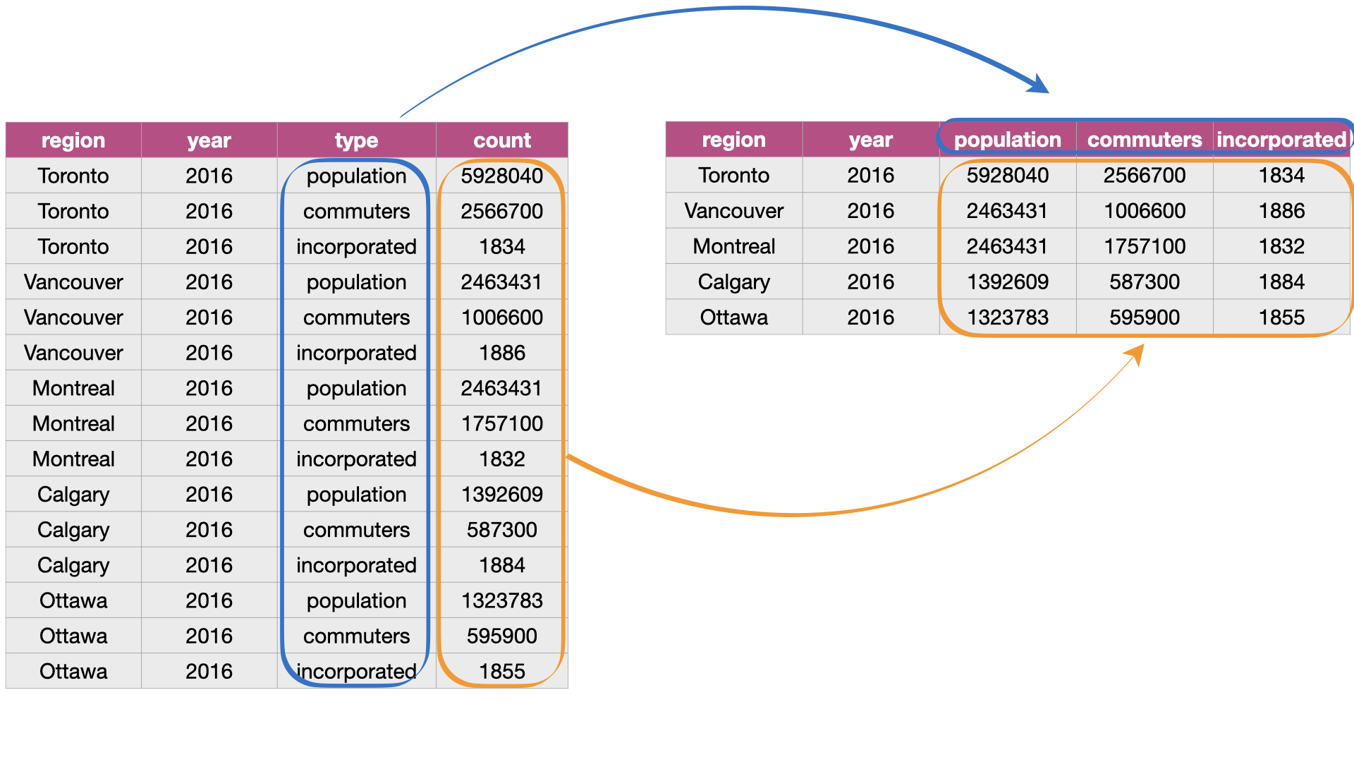
Fig. 19 Going from long to wide data.
To tidy this type of data in Python, we can use the .pivot function.
The .pivot function generally increases the number of columns (widens)
and decreases the number of rows in a data set.
To learn how to use .pivot,
we will work through an example
with the region_lang_top5_cities_long.csv data set.
This data set contains the number of Canadians reporting
the primary language at home and work for five
major cities (Toronto, Montréal, Vancouver, Calgary and Edmonton).
lang_long = pd.read_csv("data/region_lang_top5_cities_long.csv")
lang_long
| region | category | language | type | count | |
|---|---|---|---|---|---|
| 0 | Montréal | Aboriginal languages | Aboriginal languages, n.o.s. | most_at_home | 15 |
| 1 | Montréal | Aboriginal languages | Aboriginal languages, n.o.s. | most_at_work | 0 |
| 2 | Toronto | Aboriginal languages | Aboriginal languages, n.o.s. | most_at_home | 50 |
| 3 | Toronto | Aboriginal languages | Aboriginal languages, n.o.s. | most_at_work | 0 |
| 4 | Calgary | Aboriginal languages | Aboriginal languages, n.o.s. | most_at_home | 5 |
| ... | ... | ... | ... | ... | ... |
| 2135 | Calgary | Non-Official & Non-Aboriginal languages | Yoruba | most_at_work | 0 |
| 2136 | Edmonton | Non-Official & Non-Aboriginal languages | Yoruba | most_at_home | 280 |
| 2137 | Edmonton | Non-Official & Non-Aboriginal languages | Yoruba | most_at_work | 0 |
| 2138 | Vancouver | Non-Official & Non-Aboriginal languages | Yoruba | most_at_home | 40 |
| 2139 | Vancouver | Non-Official & Non-Aboriginal languages | Yoruba | most_at_work | 0 |
2140 rows × 5 columns
What makes the data set shown above untidy?
In this example, each observation is a language in a region.
However, each observation is split across multiple rows:
one where the count for most_at_home is recorded,
and the other where the count for most_at_work is recorded.
Suppose the goal with this data was to
visualize the relationship between the number of
Canadians reporting their primary language at home and work.
Doing that would be difficult with this data in its current form,
since these two variables are stored in the same column.
Fig. 20 shows how this data
will be tidied using the .pivot function.
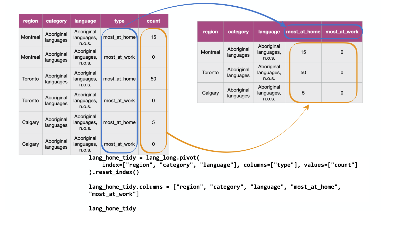
Fig. 20 Going from long to wide with the .pivot function.
Fig. 21 details the arguments that we need to specify
in the .pivot function.
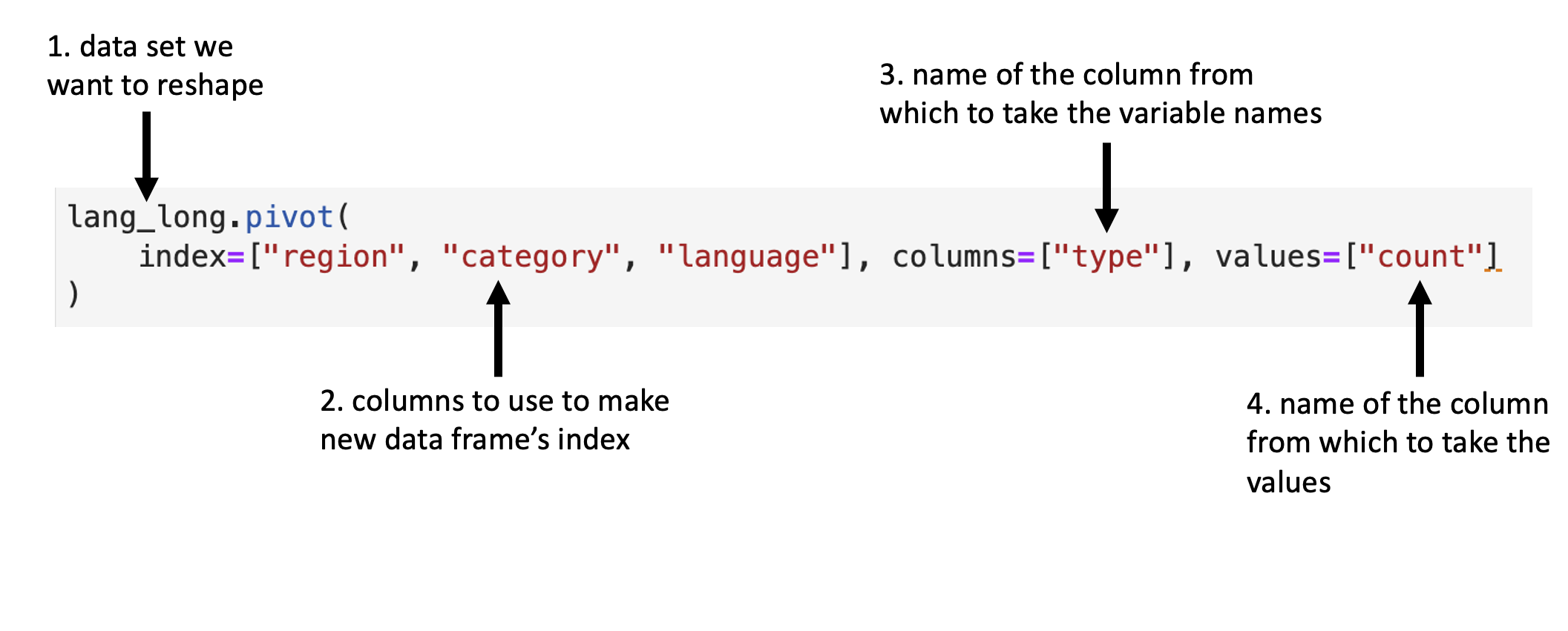
Fig. 21 Syntax for the .pivot function.
We will apply the function as detailed in Fig. 21.
lang_home_tidy = lang_long.pivot(
    index=["region", "category", "language"], columns=["type"], values=["count"]
).reset_index()

lang_home_tidy.columns = [
    "region",
    "category",
    "language",
    "most_at_home",
    "most_at_work",
]
lang_home_tidy
| region | category | language | most_at_home | most_at_work | |
|---|---|---|---|---|---|
| 0 | Calgary | Aboriginal languages | Aboriginal languages, n.o.s. | 5 | 0 |
| 1 | Calgary | Aboriginal languages | Algonquian languages, n.i.e. | 0 | 0 |
| 2 | Calgary | Aboriginal languages | Algonquin | 0 | 0 |
| 3 | Calgary | Aboriginal languages | Athabaskan languages, n.i.e. | 0 | 0 |
| 4 | Calgary | Aboriginal languages | Atikamekw | 0 | 0 |
| ... | ... | ... | ... | ... | ... |
| 1065 | Vancouver | Non-Official & Non-Aboriginal languages | Wu (Shanghainese) | 2495 | 45 |
| 1066 | Vancouver | Non-Official & Non-Aboriginal languages | Yiddish | 10 | 0 |
| 1067 | Vancouver | Non-Official & Non-Aboriginal languages | Yoruba | 40 | 0 |
| 1068 | Vancouver | Official languages | English | 1622735 | 1330555 |
| 1069 | Vancouver | Official languages | French | 8630 | 3245 |
1070 rows × 5 columns
lang_home_tidy.dtypes
region          object
category        object
language        object
most_at_home     int64
most_at_work     int64
dtype: object
The data above is now tidy! We can go through the three criteria again to check that this data is a tidy data set.
All the statistical variables are their own columns in the data frame (i.e.,
most_at_home, andmost_at_workhave been separated into their own columns in the data frame).Each observation, (i.e., each language in a region) is in a single row.
Each value is a single cell (i.e., its row, column position in the data frame is not shared with another value).
You might notice that we have the same number of columns in the tidy data set as
we did in the messy one. Therefore .pivot didn’t really “widen” the data.
This is just because the original type column only had
two categories in it. If it had more than two, .pivot would have created
more columns, and we would see the data set “widen.”
Tidying up: using .str.split to deal with multiple delimiters
Data are also not considered tidy when multiple values are stored in the same \index{separate}
cell. The data set we show below is even messier than the ones we dealt with
above: the Toronto, Montréal, Vancouver, Calgary and Edmonton columns
contain the number of Canadians reporting their primary language at home and
work in one column separated by the delimiter (/). The column names are the \index{delimiter}
values of a variable, and each value does not have its own cell! To turn this
messy data into tidy data, we’ll have to fix these issues.
lang_messy = pd.read_csv("data/region_lang_top5_cities_messy.csv")
lang_messy
| category | language | Toronto | Montréal | Vancouver | Calgary | Edmonton | |
|---|---|---|---|---|---|---|---|
| 0 | Aboriginal languages | Aboriginal languages, n.o.s. | 50/0 | 15/0 | 15/0 | 5/0 | 10/0 |
| 1 | Non-Official & Non-Aboriginal languages | Afrikaans | 265/0 | 10/0 | 520/10 | 505/15 | 300/0 |
| 2 | Non-Official & Non-Aboriginal languages | Afro-Asiatic languages, n.i.e. | 185/10 | 65/0 | 10/0 | 15/0 | 20/0 |
| 3 | Non-Official & Non-Aboriginal languages | Akan (Twi) | 4045/20 | 440/0 | 125/10 | 330/0 | 445/0 |
| 4 | Non-Official & Non-Aboriginal languages | Albanian | 6380/215 | 1445/20 | 530/10 | 620/25 | 370/10 |
| ... | ... | ... | ... | ... | ... | ... | ... |
| 209 | Non-Official & Non-Aboriginal languages | Wolof | 75/0 | 770/0 | 5/0 | 65/0 | 90/10 |
| 210 | Aboriginal languages | Woods Cree | 0/10 | 0/0 | 5/0 | 0/0 | 20/0 |
| 211 | Non-Official & Non-Aboriginal languages | Wu (Shanghainese) | 3130/30 | 760/15 | 2495/45 | 210/0 | 120/0 |
| 212 | Non-Official & Non-Aboriginal languages | Yiddish | 350/20 | 6665/860 | 10/0 | 10/0 | 0/0 |
| 213 | Non-Official & Non-Aboriginal languages | Yoruba | 1080/10 | 45/0 | 40/0 | 350/0 | 280/0 |
214 rows × 7 columns
First we’ll use .melt to create two columns, region and value,
similar to what we did previously.
The new region columns will contain the region names,
and the new column value will be a temporary holding place for the
data that we need to further separate, i.e., the
number of Canadians reporting their primary language at home and work.
lang_messy_longer = lang_messy.melt(
    id_vars=["category", "language"],
    value_vars=["Toronto", "Montréal", "Vancouver", "Calgary", "Edmonton"],
    var_name="region",
    value_name="value",
)

lang_messy_longer
| category | language | region | value | |
|---|---|---|---|---|
| 0 | Aboriginal languages | Aboriginal languages, n.o.s. | Toronto | 50/0 |
| 1 | Non-Official & Non-Aboriginal languages | Afrikaans | Toronto | 265/0 |
| 2 | Non-Official & Non-Aboriginal languages | Afro-Asiatic languages, n.i.e. | Toronto | 185/10 |
| 3 | Non-Official & Non-Aboriginal languages | Akan (Twi) | Toronto | 4045/20 |
| 4 | Non-Official & Non-Aboriginal languages | Albanian | Toronto | 6380/215 |
| ... | ... | ... | ... | ... |
| 1065 | Non-Official & Non-Aboriginal languages | Wolof | Edmonton | 90/10 |
| 1066 | Aboriginal languages | Woods Cree | Edmonton | 20/0 |
| 1067 | Non-Official & Non-Aboriginal languages | Wu (Shanghainese) | Edmonton | 120/0 |
| 1068 | Non-Official & Non-Aboriginal languages | Yiddish | Edmonton | 0/0 |
| 1069 | Non-Official & Non-Aboriginal languages | Yoruba | Edmonton | 280/0 |
1070 rows × 4 columns
Next we’ll use .str.split to split the value column into two columns.
One column will contain only the counts of Canadians
that speak each language most at home,
and the other will contain the counts of Canadians
that speak each language most at work for each region.
Fig. 22
outlines what we need to specify to use .str.split.
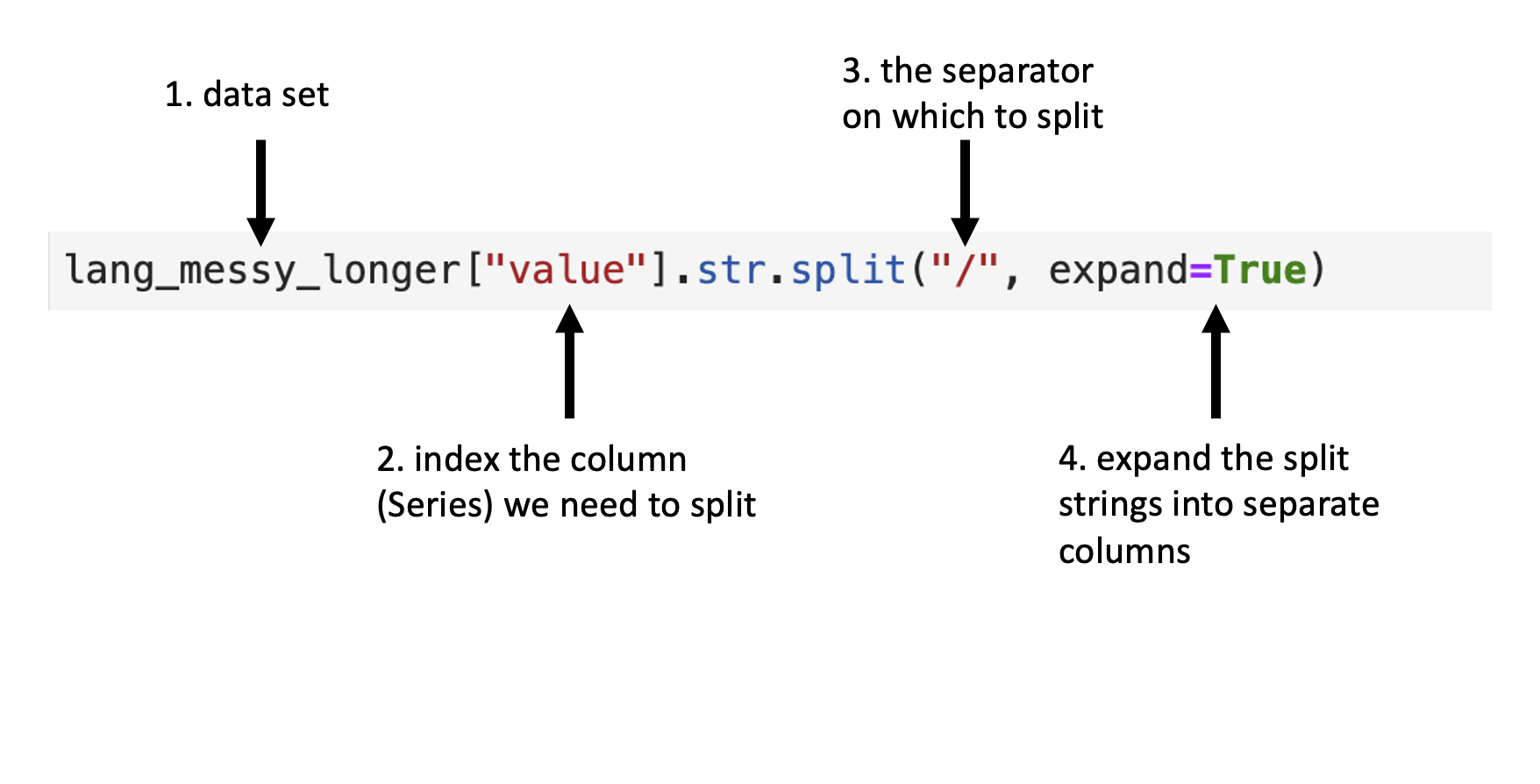
Fig. 22 Syntax for the .str.split function.
tidy_lang = (
    pd.concat(
        (lang_messy_longer, lang_messy_longer["value"].str.split("/", expand=True)),
        axis=1,
    )
    .rename(columns={0: "most_at_home", 1: "most_at_work"})
    .drop(columns=["value"])
)

tidy_lang
| category | language | region | most_at_home | most_at_work | |
|---|---|---|---|---|---|
| 0 | Aboriginal languages | Aboriginal languages, n.o.s. | Toronto | 50 | 0 |
| 1 | Non-Official & Non-Aboriginal languages | Afrikaans | Toronto | 265 | 0 |
| 2 | Non-Official & Non-Aboriginal languages | Afro-Asiatic languages, n.i.e. | Toronto | 185 | 10 |
| 3 | Non-Official & Non-Aboriginal languages | Akan (Twi) | Toronto | 4045 | 20 |
| 4 | Non-Official & Non-Aboriginal languages | Albanian | Toronto | 6380 | 215 |
| ... | ... | ... | ... | ... | ... |
| 1065 | Non-Official & Non-Aboriginal languages | Wolof | Edmonton | 90 | 10 |
| 1066 | Aboriginal languages | Woods Cree | Edmonton | 20 | 0 |
| 1067 | Non-Official & Non-Aboriginal languages | Wu (Shanghainese) | Edmonton | 120 | 0 |
| 1068 | Non-Official & Non-Aboriginal languages | Yiddish | Edmonton | 0 | 0 |
| 1069 | Non-Official & Non-Aboriginal languages | Yoruba | Edmonton | 280 | 0 |
1070 rows × 5 columns
tidy_lang.dtypes
category        object
language        object
region          object
most_at_home    object
most_at_work    object
dtype: object
Is this data set now tidy? If we recall the three criteria for tidy data:
each row is a single observation,
each column is a single variable, and
each value is a single cell.
We can see that this data now satisfies all three criteria, making it easier to
analyze. But we aren’t done yet! Notice in the table, all of the variables are
“object” data types. Object data types are columns of strings or columns with mixed types. In the previous example in Section Tidying up: going from long to wide using .pivot, the
most_at_home and most_at_work variables were int64 (integer)—you can
verify this by calling df.dtypes—which is a type
of numeric data. This change is due to the delimiter (/) when we read in this
messy data set. Python read these columns in as string types, and by default,
.str.split will return columns as object data types.
It makes sense for region, category, and language to be stored as a
object type. However, suppose we want to apply any functions that treat the
most_at_home and most_at_work columns as a number (e.g., finding rows
above a numeric threshold of a column).
In that case,
it won’t be possible to do if the variable is stored as a object.
Fortunately, the pandas.to_numeric function provides a natural way to fix problems
like this: it will convert the columns to the best numeric data types.
tidy_lang["most_at_home"] = pd.to_numeric(tidy_lang["most_at_home"])
tidy_lang["most_at_work"] = pd.to_numeric(tidy_lang["most_at_work"])
tidy_lang
| category | language | region | most_at_home | most_at_work | |
|---|---|---|---|---|---|
| 0 | Aboriginal languages | Aboriginal languages, n.o.s. | Toronto | 50 | 0 |
| 1 | Non-Official & Non-Aboriginal languages | Afrikaans | Toronto | 265 | 0 |
| 2 | Non-Official & Non-Aboriginal languages | Afro-Asiatic languages, n.i.e. | Toronto | 185 | 10 |
| 3 | Non-Official & Non-Aboriginal languages | Akan (Twi) | Toronto | 4045 | 20 |
| 4 | Non-Official & Non-Aboriginal languages | Albanian | Toronto | 6380 | 215 |
| ... | ... | ... | ... | ... | ... |
| 1065 | Non-Official & Non-Aboriginal languages | Wolof | Edmonton | 90 | 10 |
| 1066 | Aboriginal languages | Woods Cree | Edmonton | 20 | 0 |
| 1067 | Non-Official & Non-Aboriginal languages | Wu (Shanghainese) | Edmonton | 120 | 0 |
| 1068 | Non-Official & Non-Aboriginal languages | Yiddish | Edmonton | 0 | 0 |
| 1069 | Non-Official & Non-Aboriginal languages | Yoruba | Edmonton | 280 | 0 |
1070 rows × 5 columns
tidy_lang.dtypes
category        object
language        object
region          object
most_at_home     int64
most_at_work     int64
dtype: object
Now we see most_at_home and most_at_work columns are of int64 data types,
indicating they are integer data types (i.e., numbers)!
Using .loc[] and .iloc[] to extract a range of columns
Now that the tidy_lang data is indeed tidy, we can start manipulating it \index{select!helpers}
using the powerful suite of functions from the pandas.
For the first example, recall .loc[] from Chapter intro,
which lets us create a subset of columns from a data frame.
Suppose we wanted to select only the columns language, region,
most_at_home and most_at_work from the tidy_lang data set. Using what we
learned in Chapter intro, we would pass all of these column names into the square brackets:
selected_columns = tidy_lang.loc[:, ["language", "region", "most_at_home", "most_at_work"]]
selected_columns
| language | region | most_at_home | most_at_work | |
|---|---|---|---|---|
| 0 | Aboriginal languages, n.o.s. | Toronto | 50 | 0 |
| 1 | Afrikaans | Toronto | 265 | 0 |
| 2 | Afro-Asiatic languages, n.i.e. | Toronto | 185 | 10 |
| 3 | Akan (Twi) | Toronto | 4045 | 20 |
| 4 | Albanian | Toronto | 6380 | 215 |
| ... | ... | ... | ... | ... |
| 1065 | Wolof | Edmonton | 90 | 10 |
| 1066 | Woods Cree | Edmonton | 20 | 0 |
| 1067 | Wu (Shanghainese) | Edmonton | 120 | 0 |
| 1068 | Yiddish | Edmonton | 0 | 0 |
| 1069 | Yoruba | Edmonton | 280 | 0 |
1070 rows × 4 columns
Here we wrote out the names of each of the columns. However, this method is
time-consuming, especially if you have a lot of columns! Another approach is to
index with integers. .iloc[] make it easier for
us to select columns. For instance, we can use .iloc[] to choose a
range of columns rather than typing each column name out. To do this, we use the
colon (:) operator to denote the range. For example, to get all the columns in \index{column range}
the tidy_lang data frame from language to most_at_work, we pass : before the comma indicating we want to retrieve all rows, and 1: after the comma indicating we want only columns from index 1 (i.e. language) and afterwords.
column_range = tidy_lang.iloc[:, 1:]
column_range
| language | region | most_at_home | most_at_work | |
|---|---|---|---|---|
| 0 | Aboriginal languages, n.o.s. | Toronto | 50 | 0 |
| 1 | Afrikaans | Toronto | 265 | 0 |
| 2 | Afro-Asiatic languages, n.i.e. | Toronto | 185 | 10 |
| 3 | Akan (Twi) | Toronto | 4045 | 20 |
| 4 | Albanian | Toronto | 6380 | 215 |
| ... | ... | ... | ... | ... |
| 1065 | Wolof | Edmonton | 90 | 10 |
| 1066 | Woods Cree | Edmonton | 20 | 0 |
| 1067 | Wu (Shanghainese) | Edmonton | 120 | 0 |
| 1068 | Yiddish | Edmonton | 0 | 0 |
| 1069 | Yoruba | Edmonton | 280 | 0 |
1070 rows × 4 columns
Notice that we get the same output as we did above, but with less (and clearer!) code. This type of operator is especially handy for large data sets.
Suppose instead we wanted to extract columns that followed a particular pattern
rather than just selecting a range. For example, let’s say we wanted only to select the
columns most_at_home and most_at_work. There are other functions that allow
us to select variables based on their names. In particular, we can use the .str.startswith method \index{select!starts_with}
to choose only the columns that start with the word “most”:
tidy_lang.loc[:, tidy_lang.columns.str.startswith('most')]
| most_at_home | most_at_work | |
|---|---|---|
| 0 | 50 | 0 |
| 1 | 265 | 0 |
| 2 | 185 | 10 |
| 3 | 4045 | 20 |
| 4 | 6380 | 215 |
| ... | ... | ... |
| 1065 | 90 | 10 |
| 1066 | 20 | 0 |
| 1067 | 120 | 0 |
| 1068 | 0 | 0 |
| 1069 | 280 | 0 |
1070 rows × 2 columns
We could also have chosen the columns containing an underscore _ by using the
.str.contains("_"), since we notice
the columns we want contain underscores and the others don’t. \index{select!contains}
tidy_lang.loc[:, tidy_lang.columns.str.contains('_')]
| most_at_home | most_at_work | |
|---|---|---|
| 0 | 50 | 0 |
| 1 | 265 | 0 |
| 2 | 185 | 10 |
| 3 | 4045 | 20 |
| 4 | 6380 | 215 |
| ... | ... | ... |
| 1065 | 90 | 10 |
| 1066 | 20 | 0 |
| 1067 | 120 | 0 |
| 1068 | 0 | 0 |
| 1069 | 280 | 0 |
1070 rows × 2 columns
There are many different functions that help with selecting variables based on certain criteria. The additional resources section at the end of this chapter provides a comprehensive resource on these functions.
Using df[] to extract rows
Next, we revisit the df[] from Chapter intro,
which lets us create a subset of rows from a data frame.
Recall the argument to the df[]:
column names or a logical statement evaluated to either True or False;
df[] works by returning the rows where the logical statement evaluates to True.
This section will highlight more advanced usage of the df[] function.
In particular, this section provides an in-depth treatment of the variety of logical statements
one can use in the df[] to select subsets of rows.
Extracting rows that have a certain value with ==
Suppose we are only interested in the subset of rows in tidy_lang corresponding to the
official languages of Canada (English and French).
We can extract these rows by using the equivalency operator (==)
to compare the values of the category column
with the value "Official languages".
With these arguments, df[] returns a data frame with all the columns
of the input data frame
but only the rows we asked for in the logical statement, i.e.,
those where the category column holds the value "Official languages".
We name this data frame official_langs.
official_langs = tidy_lang[tidy_lang["category"] == "Official languages"]
official_langs
| category | language | region | most_at_home | most_at_work | |
|---|---|---|---|---|---|
| 54 | Official languages | English | Toronto | 3836770 | 3218725 |
| 59 | Official languages | French | Toronto | 29800 | 11940 |
| 268 | Official languages | English | Montréal | 620510 | 412120 |
| 273 | Official languages | French | Montréal | 2669195 | 1607550 |
| 482 | Official languages | English | Vancouver | 1622735 | 1330555 |
| 487 | Official languages | French | Vancouver | 8630 | 3245 |
| 696 | Official languages | English | Calgary | 1065070 | 844740 |
| 701 | Official languages | French | Calgary | 8630 | 2140 |
| 910 | Official languages | English | Edmonton | 1050410 | 792700 |
| 915 | Official languages | French | Edmonton | 10950 | 2520 |
Extracting rows that do not have a certain value with !=
What if we want all the other language categories in the data set except for
those in the "Official languages" category? We can accomplish this with the !=
operator, which means “not equal to”. So if we want to find all the rows
where the category does not equal "Official languages" we write the code
below.
tidy_lang[tidy_lang["category"] != "Official languages"]
| category | language | region | most_at_home | most_at_work | |
|---|---|---|---|---|---|
| 0 | Aboriginal languages | Aboriginal languages, n.o.s. | Toronto | 50 | 0 |
| 1 | Non-Official & Non-Aboriginal languages | Afrikaans | Toronto | 265 | 0 |
| 2 | Non-Official & Non-Aboriginal languages | Afro-Asiatic languages, n.i.e. | Toronto | 185 | 10 |
| 3 | Non-Official & Non-Aboriginal languages | Akan (Twi) | Toronto | 4045 | 20 |
| 4 | Non-Official & Non-Aboriginal languages | Albanian | Toronto | 6380 | 215 |
| ... | ... | ... | ... | ... | ... |
| 1065 | Non-Official & Non-Aboriginal languages | Wolof | Edmonton | 90 | 10 |
| 1066 | Aboriginal languages | Woods Cree | Edmonton | 20 | 0 |
| 1067 | Non-Official & Non-Aboriginal languages | Wu (Shanghainese) | Edmonton | 120 | 0 |
| 1068 | Non-Official & Non-Aboriginal languages | Yiddish | Edmonton | 0 | 0 |
| 1069 | Non-Official & Non-Aboriginal languages | Yoruba | Edmonton | 280 | 0 |
1060 rows × 5 columns
Extracting rows satisfying multiple conditions using &
Suppose now we want to look at only the rows
for the French language in Montréal.
To do this, we need to filter the data set
to find rows that satisfy multiple conditions simultaneously.
We can do this with the ampersand symbol (&), which
is interpreted by Python as “and”.
We write the code as shown below to filter the official_langs data frame
to subset the rows where region == "Montréal"
and the language == "French".
tidy_lang[(tidy_lang["region"] == "Montréal") & (tidy_lang["language"] == "French")]
| category | language | region | most_at_home | most_at_work | |
|---|---|---|---|---|---|
| 273 | Official languages | French | Montréal | 2669195 | 1607550 |
Extracting rows satisfying at least one condition using |
Suppose we were interested in only those rows corresponding to cities in Alberta
in the official_langs data set (Edmonton and Calgary).
We can’t use & as we did above because region
cannot be both Edmonton and Calgary simultaneously.
Instead, we can use the vertical pipe (|) logical operator,
which gives us the cases where one condition or
another condition or both are satisfied.
In the code below, we ask Python to return the rows
where the region columns are equal to “Calgary” or “Edmonton”.
official_langs[
    (official_langs["region"] == "Calgary") | (official_langs["region"] == "Edmonton")
]
| category | language | region | most_at_home | most_at_work | |
|---|---|---|---|---|---|
| 696 | Official languages | English | Calgary | 1065070 | 844740 |
| 701 | Official languages | French | Calgary | 8630 | 2140 |
| 910 | Official languages | English | Edmonton | 1050410 | 792700 |
| 915 | Official languages | French | Edmonton | 10950 | 2520 |
Extracting rows with values in a list using .isin()
Next, suppose we want to see the populations of our five cities.
Let’s read in the region_data.csv file
that comes from the 2016 Canadian census,
as it contains statistics for number of households, land area, population
and number of dwellings for different regions.
region_data = pd.read_csv("data/region_data.csv")
region_data
| region | households | area | population | dwellings | |
|---|---|---|---|---|---|
| 0 | Belleville | 43002 | 1354.65121 | 103472 | 45050 |
| 1 | Lethbridge | 45696 | 3046.69699 | 117394 | 48317 |
| 2 | Thunder Bay | 52545 | 2618.26318 | 121621 | 57146 |
| 3 | Peterborough | 50533 | 1636.98336 | 121721 | 55662 |
| 4 | Saint John | 52872 | 3793.42158 | 126202 | 58398 |
| ... | ... | ... | ... | ... | ... |
| 30 | Ottawa - Gatineau | 535499 | 7168.96442 | 1323783 | 571146 |
| 31 | Calgary | 519693 | 5241.70103 | 1392609 | 544870 |
| 32 | Vancouver | 960894 | 3040.41532 | 2463431 | 1027613 |
| 33 | Montréal | 1727310 | 4638.24059 | 4098927 | 1823281 |
| 34 | Toronto | 2135909 | 6269.93132 | 5928040 | 2235145 |
35 rows × 5 columns
To get the population of the five cities
we can filter the data set using the .isin method.
The .isin method is used to see if an element belongs to a list.
Here we are filtering for rows where the value in the region column
matches any of the five cities we are intersted in: Toronto, Montréal,
Vancouver, Calgary, and Edmonton.
city_names = ["Toronto", "Montréal", "Vancouver", "Calgary", "Edmonton"]
five_cities = region_data[region_data["region"].isin(city_names)]
five_cities
| region | households | area | population | dwellings | |
|---|---|---|---|---|---|
| 29 | Edmonton | 502143 | 9857.77908 | 1321426 | 537634 |
| 31 | Calgary | 519693 | 5241.70103 | 1392609 | 544870 |
| 32 | Vancouver | 960894 | 3040.41532 | 2463431 | 1027613 |
| 33 | Montréal | 1727310 | 4638.24059 | 4098927 | 1823281 |
| 34 | Toronto | 2135909 | 6269.93132 | 5928040 | 2235145 |
Note: What’s the difference between
==and.isin? Suppose we have two Series,seriesAandseriesB. If you typeseriesA == seriesBinto Python it will compare the series element by element. Python checks if the first element ofseriesAequals the first element ofseriesB, the second element ofseriesAequals the second element ofseriesB, and so on. On the other hand,seriesA.isin(seriesB)compares the first element ofseriesAto all the elements inseriesB. Then the second element ofseriesAis compared to all the elements inseriesB, and so on. Notice the difference between==and.isinin the example below.
pd.Series(["Vancouver", "Toronto"]) == pd.Series(["Toronto", "Vancouver"])
0    False
1    False
dtype: bool
pd.Series(["Vancouver", "Toronto"]).isin(pd.Series(["Toronto", "Vancouver"]))
0    True
1    True
dtype: bool
Extracting rows above or below a threshold using > and <
We saw in Section Extracting rows satisfying multiple conditions using & that
2,669,195 people reported
speaking French in Montréal as their primary language at home.
If we are interested in finding the official languages in regions
with higher numbers of people who speak it as their primary language at home
compared to French in Montréal, then we can use df[] to obtain rows
where the value of most_at_home is greater than
2,669,195.
official_langs[official_langs["most_at_home"] > 2669195]
| category | language | region | most_at_home | most_at_work | |
|---|---|---|---|---|---|
| 54 | Official languages | English | Toronto | 3836770 | 3218725 |
This operation returns a data frame with only one row, indicating that when considering the official languages, only English in Toronto is reported by more people as their primary language at home than French in Montréal according to the 2016 Canadian census.
Using .assign to modify or add columns
Using .assign to modify columns
In Section Tidying up: using .str.split to deal with multiple delimiters,
when we first read in the "region_lang_top5_cities_messy.csv" data,
all of the variables were “object” data types. \index{mutate}
During the tidying process,
we used the pandas.to_numeric function
to convert the most_at_home and most_at_work columns
to the desired integer (i.e., numeric class) data types and then used df[] to overwrite columns.
But suppose we didn’t use the df[],
and needed to modify the columns some other way.
Below we create such a situation
so that we can demonstrate how to use .assign
to change the column types of a data frame.
.assign is a useful function to modify or create new data frame columns.
lang_messy = pd.read_csv("data/region_lang_top5_cities_messy.csv")
lang_messy_longer = lang_messy.melt(
    id_vars=["category", "language"],
    value_vars=["Toronto", "Montréal", "Vancouver", "Calgary", "Edmonton"],
    var_name="region",
    value_name="value",
)
tidy_lang_obj = (
    pd.concat(
        (lang_messy_longer, lang_messy_longer["value"].str.split("/", expand=True)),
        axis=1,
    )
    .rename(columns={0: "most_at_home", 1: "most_at_work"})
    .drop(columns=["value"])
)
official_langs_obj = tidy_lang_obj[tidy_lang_obj["category"] == "Official languages"]

official_langs_obj
| category | language | region | most_at_home | most_at_work | |
|---|---|---|---|---|---|
| 54 | Official languages | English | Toronto | 3836770 | 3218725 |
| 59 | Official languages | French | Toronto | 29800 | 11940 |
| 268 | Official languages | English | Montréal | 620510 | 412120 |
| 273 | Official languages | French | Montréal | 2669195 | 1607550 |
| 482 | Official languages | English | Vancouver | 1622735 | 1330555 |
| 487 | Official languages | French | Vancouver | 8630 | 3245 |
| 696 | Official languages | English | Calgary | 1065070 | 844740 |
| 701 | Official languages | French | Calgary | 8630 | 2140 |
| 910 | Official languages | English | Edmonton | 1050410 | 792700 |
| 915 | Official languages | French | Edmonton | 10950 | 2520 |
official_langs_obj.dtypes
category        object
language        object
region          object
most_at_home    object
most_at_work    object
dtype: object
To use the .assign method, again we first specify the object to be the data set,
and in the following arguments,
we specify the name of the column we want to modify or create
(here most_at_home and most_at_work), an = sign,
and then the function we want to apply (here pandas.to_numeric).
In the function we want to apply,
we refer to the column upon which we want it to act
(here most_at_home and most_at_work).
In our example, we are naming the columns the same
names as columns that already exist in the data frame
(“most_at_home”, “most_at_work”)
and this will cause .assign to overwrite those columns
(also referred to as modifying those columns in-place).
If we were to give the columns a new name,
then .assign would create new columns with the names we specified.
.assign’s general syntax is detailed in Fig. 23.
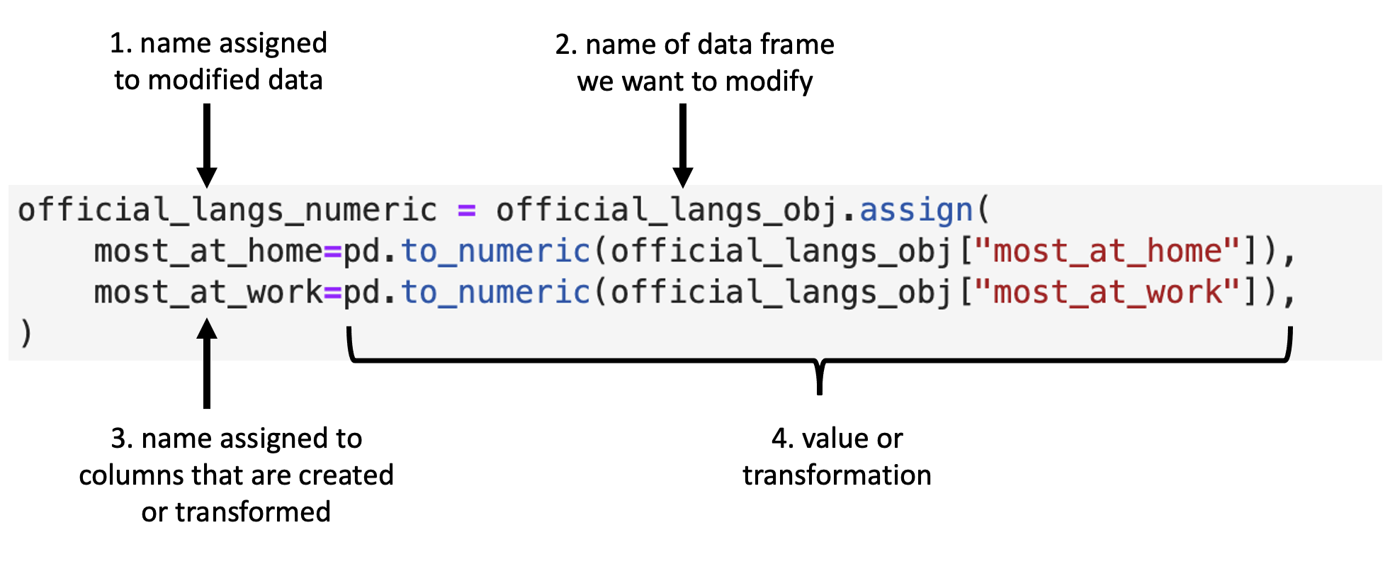
Fig. 23 Syntax for the .assign function.
Below we use .assign to convert the columns most_at_home and most_at_work
to numeric data types in the official_langs data set as described in
Fig. 23:
official_langs_numeric = official_langs_obj.assign(
    most_at_home=pd.to_numeric(official_langs_obj["most_at_home"]),
    most_at_work=pd.to_numeric(official_langs_obj["most_at_work"]),
)

official_langs_numeric
| category | language | region | most_at_home | most_at_work | |
|---|---|---|---|---|---|
| 54 | Official languages | English | Toronto | 3836770 | 3218725 |
| 59 | Official languages | French | Toronto | 29800 | 11940 |
| 268 | Official languages | English | Montréal | 620510 | 412120 |
| 273 | Official languages | French | Montréal | 2669195 | 1607550 |
| 482 | Official languages | English | Vancouver | 1622735 | 1330555 |
| 487 | Official languages | French | Vancouver | 8630 | 3245 |
| 696 | Official languages | English | Calgary | 1065070 | 844740 |
| 701 | Official languages | French | Calgary | 8630 | 2140 |
| 910 | Official languages | English | Edmonton | 1050410 | 792700 |
| 915 | Official languages | French | Edmonton | 10950 | 2520 |
official_langs_numeric.dtypes
category        object
language        object
region          object
most_at_home     int64
most_at_work     int64
dtype: object
Now we see that the most_at_home and most_at_work columns are both int64 (which is a numeric data type)!
Using .assign to create new columns
We can see in the table that 3,836,770 people reported speaking English in Toronto as their primary language at home, according to the 2016 Canadian census. What does this number mean to us? To understand this number, we need context. In particular, how many people were in Toronto when this data was collected? From the 2016 Canadian census profile, the population of Toronto was reported to be 5,928,040 people. The number of people who report that English is their primary language at home is much more meaningful when we report it in this context. We can even go a step further and transform this count to a relative frequency or proportion. We can do this by dividing the number of people reporting a given language as their primary language at home by the number of people who live in Toronto. For example, the proportion of people who reported that their primary language at home was English in the 2016 Canadian census was 0.65 in Toronto.
Let’s use .assign to create a new column in our data frame
that holds the proportion of people who speak English
for our five cities of focus in this chapter.
To accomplish this, we will need to do two tasks
beforehand:
Create a list containing the population values for the cities.
Filter the
official_langsdata frame so that we only keep the rows where the language is English.
To create a list containing the population values for the five cities
(Toronto, Montréal, Vancouver, Calgary, Edmonton),
we will use the [] (recall that we can also use list() to create a list):
city_pops = [5928040, 4098927, 2463431, 1392609, 1321426]
city_pops
[5928040, 4098927, 2463431, 1392609, 1321426]
And next, we will filter the official_langs data frame
so that we only keep the rows where the language is English.
We will name the new data frame we get from this english_langs:
english_langs = official_langs[official_langs["language"] == "English"]
english_langs
| category | language | region | most_at_home | most_at_work | |
|---|---|---|---|---|---|
| 54 | Official languages | English | Toronto | 3836770 | 3218725 |
| 268 | Official languages | English | Montréal | 620510 | 412120 |
| 482 | Official languages | English | Vancouver | 1622735 | 1330555 |
| 696 | Official languages | English | Calgary | 1065070 | 844740 |
| 910 | Official languages | English | Edmonton | 1050410 | 792700 |
Finally, we can use .assign to create a new column,
named most_at_home_proportion, that will have value that corresponds to
the proportion of people reporting English as their primary
language at home.
We will compute this by dividing the column by our vector of city populations.
english_langs = english_langs.assign(
    most_at_home_proportion=english_langs["most_at_home"] / city_pops
)

english_langs
| category | language | region | most_at_home | most_at_work | most_at_home_proportion | |
|---|---|---|---|---|---|---|
| 54 | Official languages | English | Toronto | 3836770 | 3218725 | 0.647224 |
| 268 | Official languages | English | Montréal | 620510 | 412120 | 0.151384 |
| 482 | Official languages | English | Vancouver | 1622735 | 1330555 | 0.658730 |
| 696 | Official languages | English | Calgary | 1065070 | 844740 | 0.764802 |
| 910 | Official languages | English | Edmonton | 1050410 | 792700 | 0.794906 |
In the computation above, we had to ensure that we ordered the city_pops vector in the
same order as the cities were listed in the english_langs data frame.
This is because Python will perform the division computation we did by dividing
each element of the most_at_home column by each element of the
city_pops list, matching them up by position.
Failing to do this would have resulted in the incorrect math being performed.
Note: In more advanced data wrangling, one might solve this problem in a less error-prone way though using a technique called “joins”. We link to resources that discuss this in the additional resources at the end of this chapter.
Combining functions by chaining the methods
In Python, we often have to call multiple methods in a sequence to process a data
frame. The basic ways of doing this can become quickly unreadable if there are
many steps. For example, suppose we need to perform three operations on a data
frame called data:
add a new column
new_colthat is double anotherold_col,filter for rows where another column,
other_col, is more than 5, andselect only the new column
new_colfor those rows.
One way of performing these three steps is to just write multiple lines of code, storing temporary objects as you go:
output_1 = data.assign(new_col=data["old_col"] * 2)
output_2 = output_1[output_1["other_col"] > 5]
output = output_2.loc[:, "new_col"]
This is difficult to understand for multiple reasons. The reader may be tricked
into thinking the named output_1 and output_2 objects are important for some
reason, while they are just temporary intermediate computations. Further, the
reader has to look through and find where output_1 and output_2 are used in
each subsequent line.
Chaining the sequential functions solves this problem, resulting in cleaner and easier-to-follow code. The code below accomplishes the same thing as the previous two code blocks:
output = (
    data.assign(new_col=data["old_col"] * 2)
    .query("other_col > 5")
    .loc[:, "new_col"]
)
Note: You might also have noticed that we split the function calls across lines, similar to when we did this earlier in the chapter for long function calls. Again, this is allowed and recommended, especially when the chained function calls create a long line of code. Doing this makes your code more readable. When you do this, it is important to use parentheses to tell Python that your code is continuing onto the next line.
Chaining df[] and .loc
Let’s work with the tidy tidy_lang data set from Section Tidying up: using .str.split to deal with multiple delimiters,
which contains the number of Canadians reporting their primary language at home
and work for five major cities
(Toronto, Montréal, Vancouver, Calgary, and Edmonton):
tidy_lang
| category | language | region | most_at_home | most_at_work | |
|---|---|---|---|---|---|
| 0 | Aboriginal languages | Aboriginal languages, n.o.s. | Toronto | 50 | 0 |
| 1 | Non-Official & Non-Aboriginal languages | Afrikaans | Toronto | 265 | 0 |
| 2 | Non-Official & Non-Aboriginal languages | Afro-Asiatic languages, n.i.e. | Toronto | 185 | 10 |
| 3 | Non-Official & Non-Aboriginal languages | Akan (Twi) | Toronto | 4045 | 20 |
| 4 | Non-Official & Non-Aboriginal languages | Albanian | Toronto | 6380 | 215 |
| ... | ... | ... | ... | ... | ... |
| 1065 | Non-Official & Non-Aboriginal languages | Wolof | Edmonton | 90 | 10 |
| 1066 | Aboriginal languages | Woods Cree | Edmonton | 20 | 0 |
| 1067 | Non-Official & Non-Aboriginal languages | Wu (Shanghainese) | Edmonton | 120 | 0 |
| 1068 | Non-Official & Non-Aboriginal languages | Yiddish | Edmonton | 0 | 0 |
| 1069 | Non-Official & Non-Aboriginal languages | Yoruba | Edmonton | 280 | 0 |
1070 rows × 5 columns
Suppose we want to create a subset of the data with only the languages and
counts of each language spoken most at home for the city of Vancouver. To do
this, we can use the df[] and .loc. First, we use df[] to
create a data frame called van_data that contains only values for Vancouver.
van_data = tidy_lang[tidy_lang["region"] == "Vancouver"]
van_data
| category | language | region | most_at_home | most_at_work | |
|---|---|---|---|---|---|
| 428 | Aboriginal languages | Aboriginal languages, n.o.s. | Vancouver | 15 | 0 |
| 429 | Non-Official & Non-Aboriginal languages | Afrikaans | Vancouver | 520 | 10 |
| 430 | Non-Official & Non-Aboriginal languages | Afro-Asiatic languages, n.i.e. | Vancouver | 10 | 0 |
| 431 | Non-Official & Non-Aboriginal languages | Akan (Twi) | Vancouver | 125 | 10 |
| 432 | Non-Official & Non-Aboriginal languages | Albanian | Vancouver | 530 | 10 |
| ... | ... | ... | ... | ... | ... |
| 637 | Non-Official & Non-Aboriginal languages | Wolof | Vancouver | 5 | 0 |
| 638 | Aboriginal languages | Woods Cree | Vancouver | 5 | 0 |
| 639 | Non-Official & Non-Aboriginal languages | Wu (Shanghainese) | Vancouver | 2495 | 45 |
| 640 | Non-Official & Non-Aboriginal languages | Yiddish | Vancouver | 10 | 0 |
| 641 | Non-Official & Non-Aboriginal languages | Yoruba | Vancouver | 40 | 0 |
214 rows × 5 columns
We then use .loc on this data frame to keep only the variables we want:
van_data_selected = van_data.loc[:, ["language", "most_at_home"]]
van_data_selected
| language | most_at_home | |
|---|---|---|
| 428 | Aboriginal languages, n.o.s. | 15 |
| 429 | Afrikaans | 520 |
| 430 | Afro-Asiatic languages, n.i.e. | 10 |
| 431 | Akan (Twi) | 125 |
| 432 | Albanian | 530 |
| ... | ... | ... |
| 637 | Wolof | 5 |
| 638 | Woods Cree | 5 |
| 639 | Wu (Shanghainese) | 2495 |
| 640 | Yiddish | 10 |
| 641 | Yoruba | 40 |
214 rows × 2 columns
Although this is valid code, there is a more readable approach we could take by
chaining the operations. With chaining, we do not need to create an intermediate
object to store the output from df[]. Instead, we can directly call .loc upon the
output of df[]:
van_data_selected = tidy_lang[tidy_lang["region"] == "Vancouver"].loc[
    :, ["language", "most_at_home"]
]

van_data_selected
| language | most_at_home | |
|---|---|---|
| 428 | Aboriginal languages, n.o.s. | 15 |
| 429 | Afrikaans | 520 |
| 430 | Afro-Asiatic languages, n.i.e. | 10 |
| 431 | Akan (Twi) | 125 |
| 432 | Albanian | 530 |
| ... | ... | ... |
| 637 | Wolof | 5 |
| 638 | Woods Cree | 5 |
| 639 | Wu (Shanghainese) | 2495 |
| 640 | Yiddish | 10 |
| 641 | Yoruba | 40 |
214 rows × 2 columns
As you can see, both of these approaches—with and without chaining—give us the same output, but the second approach is clearer and more readable.
Chaining more than two functions
Chaining can be used with any method in Python. Additionally, we can chain together more than two functions. For example, we can chain together three functions to:
extract rows (
df[]) to include only those where the counts of the language most spoken at home are greater than 10,000,extract only the columns (
.loc) corresponding toregion,languageandmost_at_home, andsort the data frame rows in order (
.sort_values) by counts of the language most spoken at home from smallest to largest.
As we saw in Chapter intro,
we can use the .sort_values function \index{arrange}
to order the rows in the data frame by the values of one or more columns.
Here we pass the column name most_at_home to sort the data frame rows by the values in that column, in ascending order.
large_region_lang = (
    tidy_lang[tidy_lang["most_at_home"] > 10000]
    .loc[:, ["region", "language", "most_at_home"]]
    .sort_values(by="most_at_home")
)

large_region_lang
| region | language | most_at_home | |
|---|---|---|---|
| 865 | Edmonton | Arabic | 10590 |
| 402 | Montréal | Tamil | 10670 |
| 584 | Vancouver | Russian | 10795 |
| 1034 | Edmonton | Spanish | 10880 |
| 915 | Edmonton | French | 10950 |
| ... | ... | ... | ... |
| 910 | Edmonton | English | 1050410 |
| 696 | Calgary | English | 1065070 |
| 482 | Vancouver | English | 1622735 |
| 273 | Montréal | French | 2669195 |
| 54 | Toronto | English | 3836770 |
67 rows × 3 columns
Now that we’ve shown you chaining as an alternative to storing temporary objects and composing code, does this mean you should never store temporary objects or compose code? Not necessarily! There are times when you will still want to do these things. For example, you might store a temporary object before feeding it into a plot function so you can iteratively change the plot without having to redo all of your data transformations. Additionally, chaining many functions can be overwhelming and difficult to debug; you may want to store a temporary object midway through to inspect your result before moving on with further steps.
Aggregating data with .assign, .agg and .apply
Calculating summary statistics on whole columns
As a part of many data analyses, we need to calculate a summary value for the data (a summary statistic). \index{summarize} Examples of summary statistics we might want to calculate are the number of observations, the average/mean value for a column, the minimum value, etc. Oftentimes, this summary statistic is calculated from the values in a data frame column, or columns, as shown in Fig. 24.
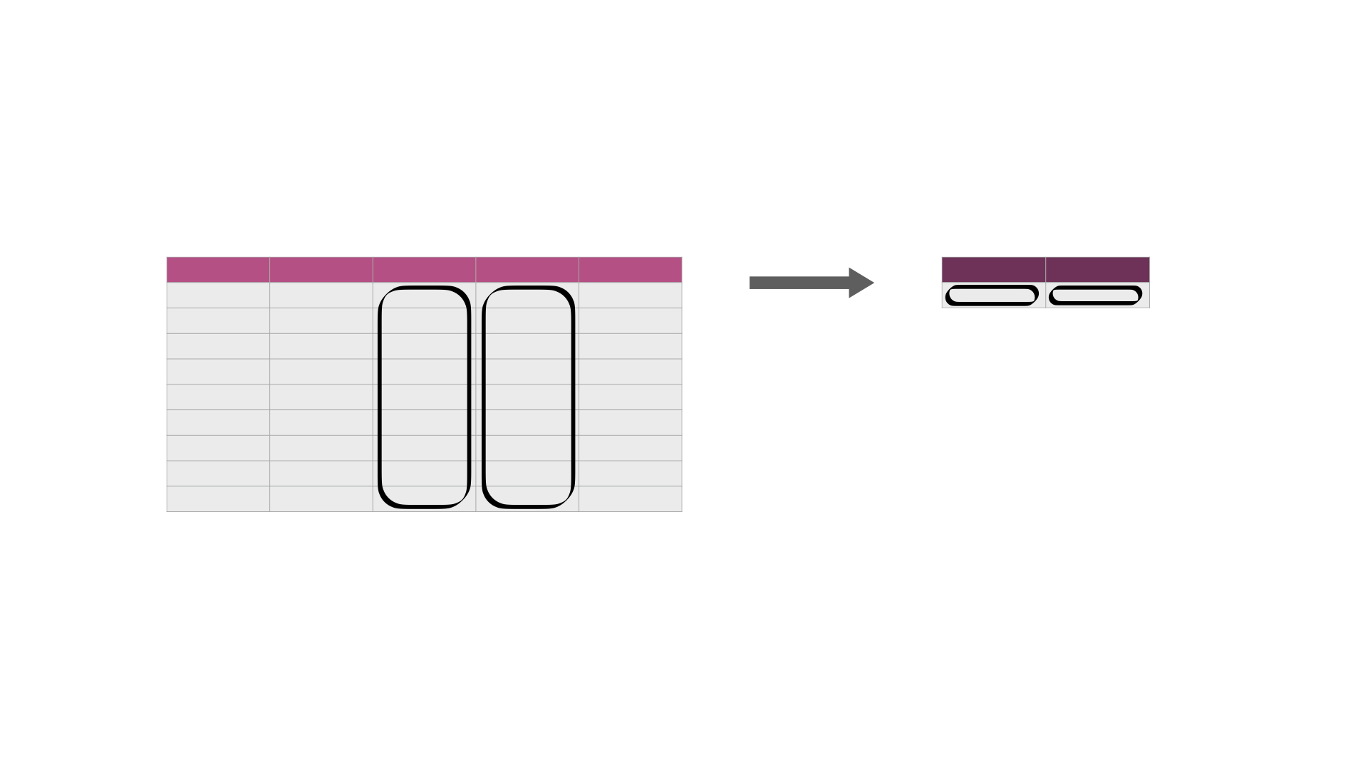
Fig. 24 Calculating summary statistics on one or more column(s). In its simplest use case, it creates a new data frame with a single row containing the summary statistic(s) for each column being summarized. The darker, top row of each table represents the column headers.
We can use .assign as mentioned in Section Using .assign to modify or add columns along with proper summary functions to create a aggregated column.
First a reminder of what region_lang looks like:
region_lang = pd.read_csv("data/region_lang.csv")
region_lang
| region | category | language | mother_tongue | most_at_home | most_at_work | lang_known | |
|---|---|---|---|---|---|---|---|
| 0 | St. John's | Aboriginal languages | Aboriginal languages, n.o.s. | 5 | 0 | 0 | 0 |
| 1 | Halifax | Aboriginal languages | Aboriginal languages, n.o.s. | 5 | 0 | 0 | 0 |
| 2 | Moncton | Aboriginal languages | Aboriginal languages, n.o.s. | 0 | 0 | 0 | 0 |
| 3 | Saint John | Aboriginal languages | Aboriginal languages, n.o.s. | 0 | 0 | 0 | 0 |
| 4 | Saguenay | Aboriginal languages | Aboriginal languages, n.o.s. | 5 | 5 | 0 | 0 |
| ... | ... | ... | ... | ... | ... | ... | ... |
| 7485 | Ottawa - Gatineau | Non-Official & Non-Aboriginal languages | Yoruba | 265 | 65 | 10 | 910 |
| 7486 | Kelowna | Non-Official & Non-Aboriginal languages | Yoruba | 5 | 0 | 0 | 0 |
| 7487 | Abbotsford - Mission | Non-Official & Non-Aboriginal languages | Yoruba | 20 | 0 | 0 | 50 |
| 7488 | Vancouver | Non-Official & Non-Aboriginal languages | Yoruba | 190 | 40 | 0 | 505 |
| 7489 | Victoria | Non-Official & Non-Aboriginal languages | Yoruba | 20 | 0 | 0 | 90 |
7490 rows × 7 columns
We apply min to calculate the minimum
and max to calculate maximum number of Canadians
reporting a particular language as their primary language at home,
for any region, and .assign a column name to each:
lang_summary = pd.DataFrame()
lang_summary = lang_summary.assign(min_most_at_home=[min(region_lang["most_at_home"])])
lang_summary = lang_summary.assign(max_most_at_home=[max(region_lang["most_at_home"])])
lang_summary
| min_most_at_home | max_most_at_home | |
|---|---|---|
| 0 | 0 | 3836770 |
From this we see that there are some languages in the data set that no one speaks as their primary language at home. We also see that the most commonly spoken primary language at home is spoken by 3,836,770 people.
Calculating summary statistics when there are NaNs
In pandas DataFrame, the value NaN is often used to denote missing data.
Many of the base python statistical summary functions
(e.g., max, min, sum, etc) will return NaN
when applied to columns containing NaN values. \index{missing data}\index{NA|see{missing data}}
Usually that is not what we want to happen;
instead, we would usually like Python to ignore the missing entries
and calculate the summary statistic using all of the other non-NaN values
in the column.
Fortunately pandas provides many equivalent methods (e.g., .max, .min, .sum, etc) to
these summary functions while providing an extra argument skipna that lets
us tell the function what to do when it encounters NaN values.
In particular, if we specify skipna=True (default), the function will ignore
missing values and return a summary of all the non-missing entries.
We show an example of this below.
First we create a new version of the region_lang data frame,
named region_lang_na, that has a seemingly innocuous NaN
in the first row of the most_at_home column:
region_lang_na
| region | category | language | mother_tongue | most_at_home | most_at_work | lang_known | |
|---|---|---|---|---|---|---|---|
| 0 | St. John's | Aboriginal languages | Aboriginal languages, n.o.s. | 5 | NaN | 0 | 0 |
| 1 | Halifax | Aboriginal languages | Aboriginal languages, n.o.s. | 5 | 0.0 | 0 | 0 |
| 2 | Moncton | Aboriginal languages | Aboriginal languages, n.o.s. | 0 | 0.0 | 0 | 0 |
| 3 | Saint John | Aboriginal languages | Aboriginal languages, n.o.s. | 0 | 0.0 | 0 | 0 |
| 4 | Saguenay | Aboriginal languages | Aboriginal languages, n.o.s. | 5 | 5.0 | 0 | 0 |
| ... | ... | ... | ... | ... | ... | ... | ... |
| 7485 | Ottawa - Gatineau | Non-Official & Non-Aboriginal languages | Yoruba | 265 | 65.0 | 10 | 910 |
| 7486 | Kelowna | Non-Official & Non-Aboriginal languages | Yoruba | 5 | 0.0 | 0 | 0 |
| 7487 | Abbotsford - Mission | Non-Official & Non-Aboriginal languages | Yoruba | 20 | 0.0 | 0 | 50 |
| 7488 | Vancouver | Non-Official & Non-Aboriginal languages | Yoruba | 190 | 40.0 | 0 | 505 |
| 7489 | Victoria | Non-Official & Non-Aboriginal languages | Yoruba | 20 | 0.0 | 0 | 90 |
7490 rows × 7 columns
Now if we apply the Python built-in summary function as above,
we see that we no longer get the minimum and maximum returned,
but just an NaN instead!
lang_summary_na = pd.DataFrame()
lang_summary_na = lang_summary_na.assign(
    min_most_at_home=[min(region_lang_na["most_at_home"])]
)
lang_summary_na = lang_summary_na.assign(
    max_most_at_home=[max(region_lang_na["most_at_home"])]
)
lang_summary_na
| min_most_at_home | max_most_at_home | |
|---|---|---|
| 0 | NaN | NaN |
We can fix this by using the pandas Series methods (i.e. .min and .max) with skipna=True as explained above:
lang_summary_na = pd.DataFrame()
lang_summary_na = lang_summary_na.assign(
    min_most_at_home=[region_lang_na["most_at_home"].min(skipna=True)]
)
lang_summary_na = lang_summary_na.assign(
    max_most_at_home=[region_lang_na["most_at_home"].max(skipna=True)]
)
lang_summary_na
| min_most_at_home | max_most_at_home | |
|---|---|---|
| 0 | 0.0 | 3836770.0 |
Calculating summary statistics for groups of rows
A common pairing with summary functions is .groupby. Pairing these functions \index{group_by}
together can let you summarize values for subgroups within a data set,
as illustrated in Fig. 25.
For example, we can use .groupby to group the regions of the tidy_lang data frame and then calculate the minimum and maximum number of Canadians
reporting the language as the primary language at home
for each of the regions in the data set.
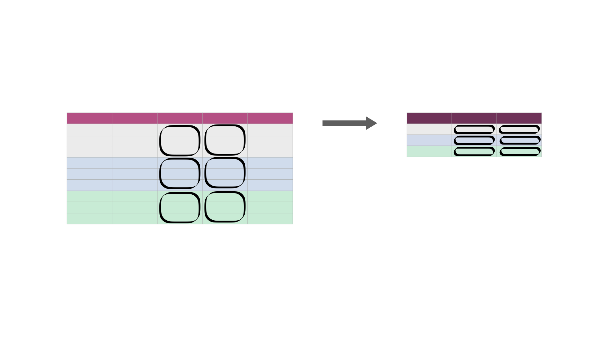
Fig. 25 Calculating summary statistics on one or more column(s) for each group. It creates a new data frame—with one row for each group—containing the summary statistic(s) for each column being summarized. It also creates a column listing the value of the grouping variable. The darker, top row of each table represents the column headers. The gray, blue, and green colored rows correspond to the rows that belong to each of the three groups being represented in this cartoon example.
The .groupby function takes at least one argument—the columns to use in the
grouping. Here we use only one column for grouping (region), but more than one
can also be used. To do this, pass a list of column names to the by argument.
region_summary = pd.DataFrame()
region_summary = region_summary.assign(
    min_most_at_home=region_lang.groupby(by="region")["most_at_home"].min(),
    max_most_at_home=region_lang.groupby(by="region")["most_at_home"].max()
).reset_index()

region_summary.columns = ["region", "min_most_at_home", "max_most_at_home"]
region_summary
| region | min_most_at_home | max_most_at_home | |
|---|---|---|---|
| 0 | Abbotsford - Mission | 0 | 137445 |
| 1 | Barrie | 0 | 182390 |
| 2 | Belleville | 0 | 97840 |
| 3 | Brantford | 0 | 124560 |
| 4 | Calgary | 0 | 1065070 |
| ... | ... | ... | ... |
| 30 | Trois-Rivières | 0 | 149835 |
| 31 | Vancouver | 0 | 1622735 |
| 32 | Victoria | 0 | 331375 |
| 33 | Windsor | 0 | 270715 |
| 34 | Winnipeg | 0 | 612595 |
35 rows × 3 columns
pandas also has a convenient method .agg (shorthand for .aggregate) that allows us to apply multiple aggregate functions in one line of code. We just need to pass in a list of function names to .agg as shown below.
region_summary = (
    region_lang.groupby(by="region")["most_at_home"].agg(["min", "max"]).reset_index()
)
region_summary.columns = ["region", "min_most_at_home", "max_most_at_home"]
region_summary
| region | min_most_at_home | max_most_at_home | |
|---|---|---|---|
| 0 | Abbotsford - Mission | 0 | 137445 |
| 1 | Barrie | 0 | 182390 |
| 2 | Belleville | 0 | 97840 |
| 3 | Brantford | 0 | 124560 |
| 4 | Calgary | 0 | 1065070 |
| ... | ... | ... | ... |
| 30 | Trois-Rivières | 0 | 149835 |
| 31 | Vancouver | 0 | 1622735 |
| 32 | Victoria | 0 | 331375 |
| 33 | Windsor | 0 | 270715 |
| 34 | Winnipeg | 0 | 612595 |
35 rows × 3 columns
Notice that .groupby converts a DataFrame object to a DataFrameGroupBy object, which contains information about the groups of the dataframe. We can then apply aggregating functions to the DataFrameGroupBy object.
region_lang.groupby("region")
<pandas.core.groupby.generic.DataFrameGroupBy object at 0x16da8ea30>
Calculating summary statistics on many columns
Sometimes we need to summarize statistics across many columns.
An example of this is illustrated in Fig. 26.
In such a case, using summary functions alone means that we have to
type out the name of each column we want to summarize.
In this section we will meet two strategies for performing this task.
First we will see how we can do this using .iloc[] to slice the columns before applying summary functions.
Then we will also explore how we can use a more general iteration function,
.apply, to also accomplish this.
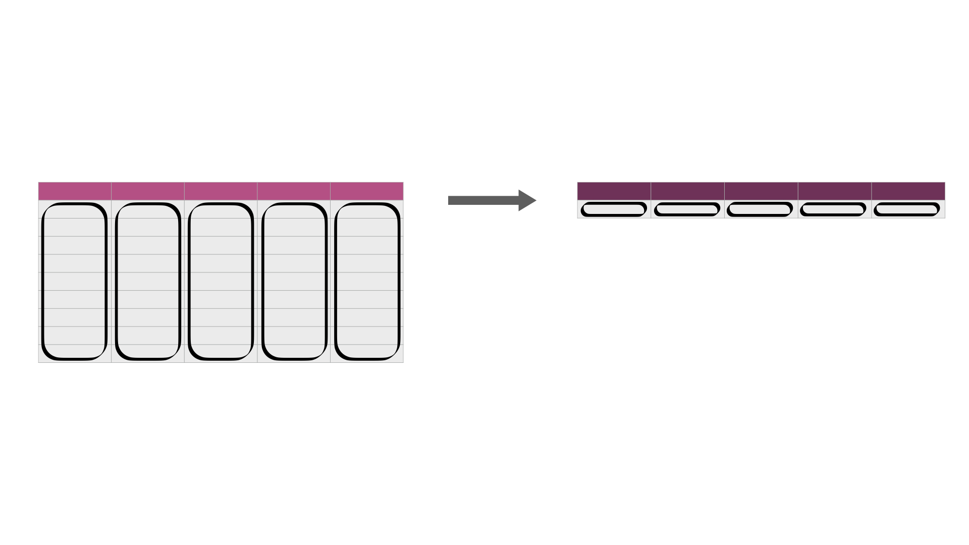
Fig. 26 .iloc[] or .apply is useful for efficiently calculating summary statistics on many columns at once. The darker, top row of each table represents the column headers.
Aggregating on a data frame for calculating summary statistics on many columns
Recall that in the Section Using .loc[] and .iloc[] to extract a range of columns, we can use .iloc[] to extract a range of columns with indices. Here we demonstrate finding the maximum value
of each of the numeric
columns of the region_lang data set through pairing .iloc[] and .max. This means that the
summary methods (e.g. .min, .max, .sum etc.) can be used for data frames as well.
pd.DataFrame(region_lang.iloc[:, 3:].max(axis=0)).T
| mother_tongue | most_at_home | most_at_work | lang_known | |
|---|---|---|---|---|
| 0 | 3061820 | 3836770 | 3218725 | 5600480 |
.apply for calculating summary statistics on many columns
An alternative to aggregating on a dataframe
for applying a function to many columns is the .apply method.
Let’s again find the maximum value of each column of the
region_lang data frame, but using .apply with the max function this time.
We focus on the two arguments of .apply:
the function that you would like to apply to each column, and the axis along which the function will be applied (0 for columns, 1 for rows).
Note that .apply does not have an argument
to specify which columns to apply the function to.
Therefore, we will use the .iloc[] before calling .apply
to choose the columns for which we want the maximum.
pd.DataFrame(region_lang.iloc[:, 3:].apply(max, axis=0)).T
| mother_tongue | most_at_home | most_at_work | lang_known | |
|---|---|---|---|---|
| 0 | 3061820 | 3836770 | 3218725 | 5600480 |
Note: Similar to when we use base Python statistical summary functions (e.g.,
max,min,sum, etc.) when there areNaNs,.applyfunctions paired with base Python statistical summary functions also returnNaNvalues when we apply them to columns that containNaNvalues. \index{missing data}To avoid this, again we need to use the
pandasvariants of summary functions (i.e..max,.min,.sum, etc.) withskipna=True. When we use this with.apply, we do this by constructing a anonymous function that calls the.maxmethod withskipna=True, as illustrated below:
pd.DataFrame(
    region_lang_na.iloc[:, 3:].apply(lambda col: col.max(skipna=True), axis=0)
).T
| mother_tongue | most_at_home | most_at_work | lang_known | |
|---|---|---|---|---|
| 0 | 3061820.0 | 3836770.0 | 3218725.0 | 5600480.0 |
The .apply function is generally quite useful for solving many problems
involving repeatedly applying functions in Python.
Additionally, a variant of .apply is .applymap,
which can be used to apply functions element-wise.
To learn more about these functions, see the additional resources
section at the end of this chapter.
Apply functions across many columns with .apply
Sometimes we need to apply a function to many columns in a data frame. For example, we would need to do this when converting units of measurements across many columns. We illustrate such a data transformation in Fig. 27.
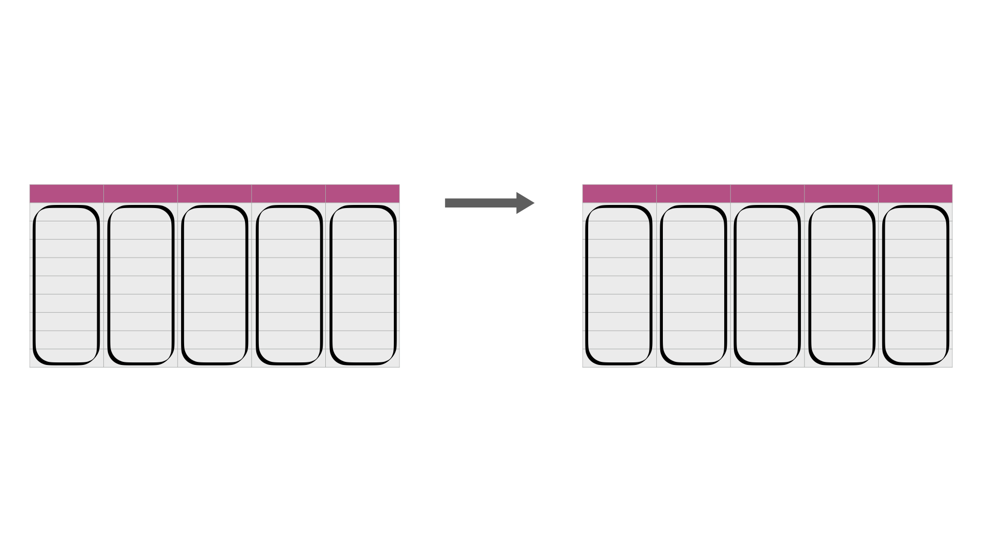
Fig. 27 .apply is useful for applying functions across many columns. The darker, top row of each table represents the column headers.
For example,
imagine that we wanted to convert all the numeric columns
in the region_lang data frame from int64 type to int32 type
using the .as_type function.
When we revisit the region_lang data frame,
we can see that this would be the columns from mother_tongue to lang_known.
region_lang
| region | category | language | mother_tongue | most_at_home | most_at_work | lang_known | |
|---|---|---|---|---|---|---|---|
| 0 | St. John's | Aboriginal languages | Aboriginal languages, n.o.s. | 5 | 0 | 0 | 0 |
| 1 | Halifax | Aboriginal languages | Aboriginal languages, n.o.s. | 5 | 0 | 0 | 0 |
| 2 | Moncton | Aboriginal languages | Aboriginal languages, n.o.s. | 0 | 0 | 0 | 0 |
| 3 | Saint John | Aboriginal languages | Aboriginal languages, n.o.s. | 0 | 0 | 0 | 0 |
| 4 | Saguenay | Aboriginal languages | Aboriginal languages, n.o.s. | 5 | 5 | 0 | 0 |
| ... | ... | ... | ... | ... | ... | ... | ... |
| 7485 | Ottawa - Gatineau | Non-Official & Non-Aboriginal languages | Yoruba | 265 | 65 | 10 | 910 |
| 7486 | Kelowna | Non-Official & Non-Aboriginal languages | Yoruba | 5 | 0 | 0 | 0 |
| 7487 | Abbotsford - Mission | Non-Official & Non-Aboriginal languages | Yoruba | 20 | 0 | 0 | 50 |
| 7488 | Vancouver | Non-Official & Non-Aboriginal languages | Yoruba | 190 | 40 | 0 | 505 |
| 7489 | Victoria | Non-Official & Non-Aboriginal languages | Yoruba | 20 | 0 | 0 | 90 |
7490 rows × 7 columns
To accomplish such a task, we can use .apply.
This works in a similar way for column selection,
as we saw when we used in Section .apply for calculating summary statistics on many columns earlier.
As we did above,
we again use .iloc to specify the columns
as well as the .apply to specify the function we want to apply on these columns.
However, a key difference here is that we are not using aggregating function here,
which means that we get back a data frame with the same number of rows.
region_lang.dtypes
region           object
category         object
language         object
mother_tongue     int64
most_at_home      int64
most_at_work      int64
lang_known        int64
dtype: object
region_lang_int32 = region_lang.iloc[:, 3:].apply(lambda col: col.astype('int32'), axis=0)
region_lang_int32 = pd.concat((region_lang.iloc[:, :3], region_lang_int32), axis=1)
region_lang_int32
| region | category | language | mother_tongue | most_at_home | most_at_work | lang_known | |
|---|---|---|---|---|---|---|---|
| 0 | St. John's | Aboriginal languages | Aboriginal languages, n.o.s. | 5 | 0 | 0 | 0 |
| 1 | Halifax | Aboriginal languages | Aboriginal languages, n.o.s. | 5 | 0 | 0 | 0 |
| 2 | Moncton | Aboriginal languages | Aboriginal languages, n.o.s. | 0 | 0 | 0 | 0 |
| 3 | Saint John | Aboriginal languages | Aboriginal languages, n.o.s. | 0 | 0 | 0 | 0 |
| 4 | Saguenay | Aboriginal languages | Aboriginal languages, n.o.s. | 5 | 5 | 0 | 0 |
| ... | ... | ... | ... | ... | ... | ... | ... |
| 7485 | Ottawa - Gatineau | Non-Official & Non-Aboriginal languages | Yoruba | 265 | 65 | 10 | 910 |
| 7486 | Kelowna | Non-Official & Non-Aboriginal languages | Yoruba | 5 | 0 | 0 | 0 |
| 7487 | Abbotsford - Mission | Non-Official & Non-Aboriginal languages | Yoruba | 20 | 0 | 0 | 50 |
| 7488 | Vancouver | Non-Official & Non-Aboriginal languages | Yoruba | 190 | 40 | 0 | 505 |
| 7489 | Victoria | Non-Official & Non-Aboriginal languages | Yoruba | 20 | 0 | 0 | 90 |
7490 rows × 7 columns
region_lang_int32.dtypes
region           object
category         object
language         object
mother_tongue     int32
most_at_home      int32
most_at_work      int32
lang_known        int32
dtype: object
We see that we get back a data frame
with the same number of columns and rows.
The only thing that changes is the transformation we applied
to the specified columns (here mother_tongue to lang_known).
Apply functions across columns within one row with .apply
What if you want to apply a function across columns but within one row? We illustrate such a data transformation in Fig. 28.
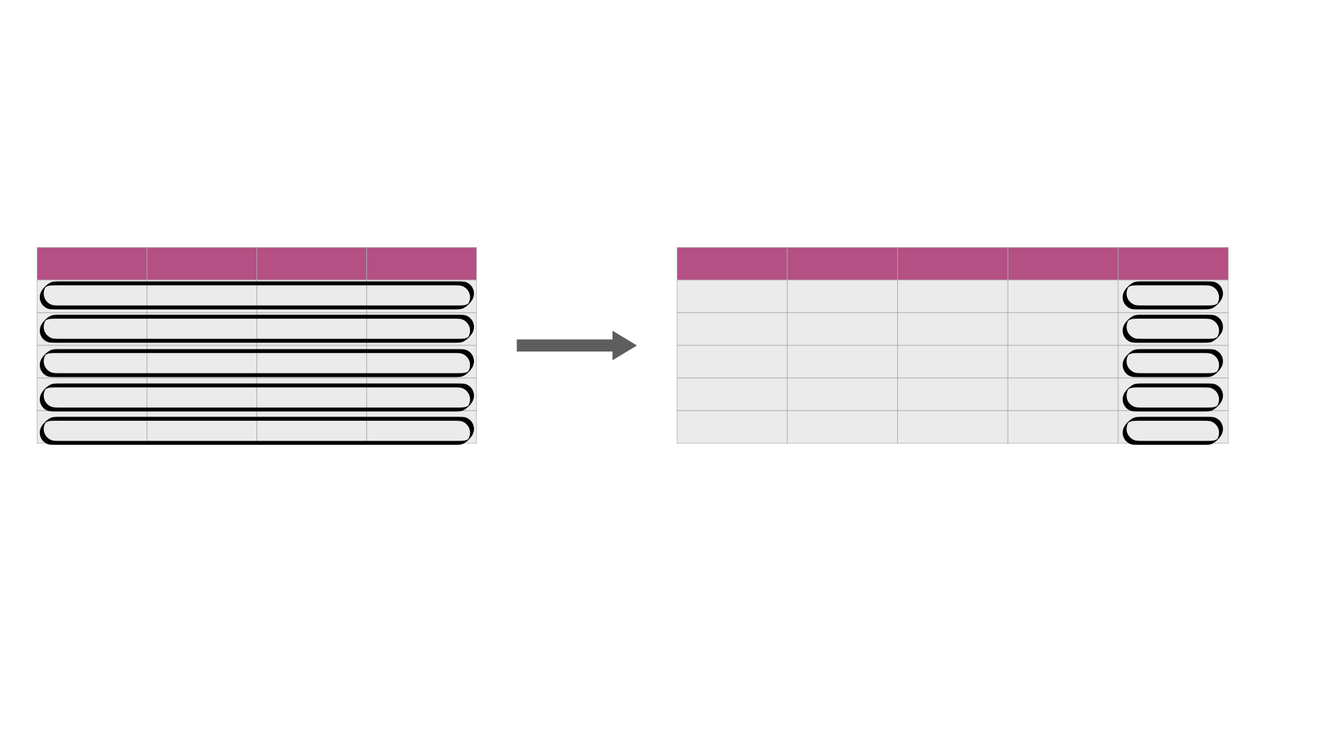
Fig. 28 .apply is useful for applying functions across columns within one row. The darker, top row of each table represents the column headers.
For instance, suppose we want to know the maximum value between mother_tongue,
most_at_home, most_at_work
and lang_known for each language and region
in the region_lang data set.
In other words, we want to apply the max function row-wise.
Before we use .apply, we will again use .iloc to select only the count columns
so we can see all the columns in the data frame’s output easily in the book.
So for this demonstration, the data set we are operating on looks like this:
region_lang.iloc[:, 3:]
| mother_tongue | most_at_home | most_at_work | lang_known | |
|---|---|---|---|---|
| 0 | 5 | 0 | 0 | 0 |
| 1 | 5 | 0 | 0 | 0 |
| 2 | 0 | 0 | 0 | 0 |
| 3 | 0 | 0 | 0 | 0 |
| 4 | 5 | 5 | 0 | 0 |
| ... | ... | ... | ... | ... |
| 7485 | 265 | 65 | 10 | 910 |
| 7486 | 5 | 0 | 0 | 0 |
| 7487 | 20 | 0 | 0 | 50 |
| 7488 | 190 | 40 | 0 | 505 |
| 7489 | 20 | 0 | 0 | 90 |
7490 rows × 4 columns
Now we use .apply with argument axis=1, to tell Python that we would like
the max function to be applied across, and within, a row,
as opposed to being applied on a column
(which is the default behavior of .apply):
region_lang_rowwise = region_lang.assign(
    maximum=region_lang.iloc[:, 3:].apply(max, axis=1)
)

region_lang_rowwise
| region | category | language | mother_tongue | most_at_home | most_at_work | lang_known | maximum | |
|---|---|---|---|---|---|---|---|---|
| 0 | St. John's | Aboriginal languages | Aboriginal languages, n.o.s. | 5 | 0 | 0 | 0 | 5 |
| 1 | Halifax | Aboriginal languages | Aboriginal languages, n.o.s. | 5 | 0 | 0 | 0 | 5 |
| 2 | Moncton | Aboriginal languages | Aboriginal languages, n.o.s. | 0 | 0 | 0 | 0 | 0 |
| 3 | Saint John | Aboriginal languages | Aboriginal languages, n.o.s. | 0 | 0 | 0 | 0 | 0 |
| 4 | Saguenay | Aboriginal languages | Aboriginal languages, n.o.s. | 5 | 5 | 0 | 0 | 5 |
| ... | ... | ... | ... | ... | ... | ... | ... | ... |
| 7485 | Ottawa - Gatineau | Non-Official & Non-Aboriginal languages | Yoruba | 265 | 65 | 10 | 910 | 910 |
| 7486 | Kelowna | Non-Official & Non-Aboriginal languages | Yoruba | 5 | 0 | 0 | 0 | 5 |
| 7487 | Abbotsford - Mission | Non-Official & Non-Aboriginal languages | Yoruba | 20 | 0 | 0 | 50 | 50 |
| 7488 | Vancouver | Non-Official & Non-Aboriginal languages | Yoruba | 190 | 40 | 0 | 505 | 505 |
| 7489 | Victoria | Non-Official & Non-Aboriginal languages | Yoruba | 20 | 0 | 0 | 90 | 90 |
7490 rows × 8 columns
We see that we get an additional column added to the data frame,
named maximum, which is the maximum value between mother_tongue,
most_at_home, most_at_work and lang_known for each language
and region.
Summary
Cleaning and wrangling data can be a very time-consuming process. However, it is a critical step in any data analysis. We have explored many different functions for cleaning and wrangling data into a tidy format. Table 5 summarizes some of the key wrangling functions we learned in this chapter. In the following chapters, you will learn how you can take this tidy data and do so much more with it to answer your burning data science questions!
Function |
Description |
|---|---|
|
calculates aggregated summaries of inputs |
|
allows you to apply function(s) to multiple columns/rows |
|
adds or modifies columns in a data frame |
|
allows you to apply function(s) to groups of rows |
|
subsets columns/rows of a data frame using integer indices |
|
subsets columns/rows of a data frame using labels |
|
generally makes the data frame longer and narrower |
|
generally makes a data frame wider and decreases the number of rows |
|
splits up a string column into multiple columns |
Exercises
Practice exercises for the material covered in this chapter can be found in the accompanying worksheets repository in the “Cleaning and wrangling data” row. You can launch an interactive version of the worksheet in your browser by clicking the “launch binder” button. You can also preview a non-interactive version of the worksheet by clicking “view worksheet.” If you instead decide to download the worksheet and run it on your own machine, make sure to follow the instructions for computer setup found in Chapter move-to-your-own-machine. This will ensure that the automated feedback and guidance that the worksheets provide will function as intended.
Additional resources
The
pandaspackage documentation is another resource to learn more about the functions in this chapter, the full set of arguments you can use, and other related functions. The site also provides a very nice cheat sheet that summarizes many of the data wrangling functions from this chapter.Python for Data Analysis [McKinney, 2012] has a few chapters related to data wrangling that go into more depth than this book. For example, the data wrangling chapter covers tidy data,
.meltand.pivot, but also covers missing values and additional wrangling functions (like.stack). The data aggregation chapter covers.groupby, aggregating functions,.apply, etc.You will occasionally encounter a case where you need to iterate over items in a data frame, but none of the above functions are flexible enough to do what you want. In that case, you may consider using a for loop [McKinney, 2012].